Archive
Distribution of number of statements in functions
The source code of individual functions is written a particular way by individuals to solve particular problems. When source code use of programming constructs are counted, in a sufficiently large quantity of source code, various patterns emerge. The most common patterns involve power laws and exponentials. The plot below shows the number of functions containing a given number of lines of code, expression-statements (e.g., assignments, calls whose return value is not used), function calls (which includes calls within an expression), and return-statements for 176,172 C functions, along with fitted power laws (data obtained using GitHub’s CodeQL variant analysis; code+data):
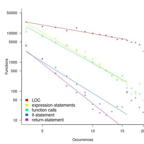
The power law exponents are: LOC 1, expression-statements 3.4, calls 3.2, if-statements 3.6, and return-statements 4.6.
This plot counts uses across all functions, to provide a global perspective. Given the quantity of data available, it’s possible to focus on the characteristics of functions containing a given number of lines of code (LOC), to study patterns of behavior that emerge as functions get longer (it was once thought that there was an optimal function length that minimised the likelihood of fault reports).
Given a function containing  LOC, what is the probability that it will contain
if-statements, or for-statements, or expression-statements, etc? The plots below show the number of if-statements that occur in 176,172 C functions containing each of 4, 5, …, 19 LOC, along with fitted regression lines (code+data):
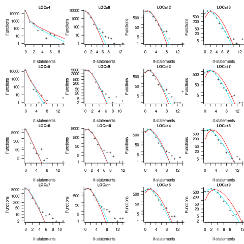
The fitted model is the probability mass function of the negative binomial distribution. The blue/green lines are individual fits to the data in each plot.
The negative binomial distribution is usually described in terms of the probability of  events occurring (or not occurring) in a sequence of
  tries, e.g., rolling two 6’s in five attempts. In a function context, this can be interpreted as the probability that there will be occurrences of a particular statement in the LOC of the function’s code.
There are various ways of specifying a negative binomial distribution. The data was fitted using R’s gamlss package, which uses the two parameters: mean ( ) and dispersion (
 ).
).
As functions get longer (i.e., LOC increases), they are more likely to contain more of each kind of statement (i.e., the mean will increase), and the variability is also likely to increase. In other words, the parameters and will increase with LOC. The red line in each plot are derived from a fitted negative binomial distribution with:  and
and  , where the values
  ,
,  ,
,  , and
, and  are returned by the fitting process (this equation was found by inspired guessing/some trial and error; another possibility is:
 , and
, and  ). This LOC dependent fits (in red) closely follow the bespoke fits (in blue/green), and for larger LOC are not affected by noisy data points.
Being able to fit a single model to the data over a range of LOCs shows that a consistent pattern of behavior exists. Similar models can be built for number of calls, while-statements, expression-statements and number of local variables. The model of for-statements suffered from high variability counts, and return-statements counts grew too slowly over the range of LOC analysed.
If the number of if-statements, say, within functions of a given size has a negative binomial distribution, then adding together all these distributions, weighted by the number of functions at a given size, should produce a power law whose exponent matches that found in the first plot (i.e., 3.6).
I asked ChatGPT: “If $y(k, x)=a*x^{-b}*NB(k; mu=log(x), sigma=log(x))$ where: $NB$ is the probability mass of the negative binomial distribution, $mu$ is its mean and $x$ takes positive integer values, $a$ is a positive constant, and $1 < b < 3$. Show that the series $sum_{x=3}^14 y(k, x)$i for $0 < k < 10$ is approximately a power law." and obtained the response that the exponent was approximately  (i.e., about 2), which is not close.
The responses from other LLMs were not any better. The calculation requires various simplifying assumptions (all the models resorted to numerical simulation at some point), and these need to be checked.
Call graph neighbourhood and fault prediction
Fault reports are generated by a program’s users, and the extreme difficulty of obtaining any information about how users use a program and number of users makes it almost impossible to do reliable fault prediction.
Source code is often available. Are there any source code characteristics that could be used to make fault predictions?
A significant number of published software fault prediction papers are based on the idea that the code contained in the functions modified to fix reported faults have ‘woo‘ characteristics that is not present in the code of other functions. Discovering these woo characteristics would make it possible to reliably predict faults. Countless hours of machine learning have been invested on the search for woo.
Faults are reported in the code that users execute, and the more often the code is executed, the more opportunities there are for fault triggering input values to occur.
Functions that have been modified to fix faults tell us something about the code that is executed by users. If a function in file A calls a function in file B which in turn calls a function in file C, and file B has be modified to fix a fault, then we know that a function in A has been called, and perhaps also in C (yes, call-chains are usually links between functions, not links between the files that contain them; most files contain only a few functions). Are files in the call-chain neighbourhood of a fault-fixed file more likely, in the future, to be modified because of a reported fault, than files that are not in such a call-chain neighbourhood?
The paper Do Bugs Propagate? An Empirical Analysis of Temporal Correlations Among Software Bugs by Gu, Han, Kim and Zhang extracted data on files/functions from multiple releases of the four systems: HTTPClient, Jackrabbit, Lucene, and Rhino, including LOC, call-graph, number of changes/authors, and number of fixed faults.
For a particular system, data on each file/function and its neighbourhood in release was then used to build a regression model that predicts the likelihood of each file needing to be changed to fix a reported fault in the next release,  .
.
The technical details of the regression fitting process for this data are more complicated than usual, and are discussed at the end of the post. The important question is whether information on call-chain neighbourhood fault reports have a worthwhile impact on the performance of a fault prediction model.
Yes, call-chain neighbourhood information does make a worthwhile improvement to fault prediction in the next release (as expected, LOC has a big impact).
The authors also built a co-change graph (i.e., files modified in the same commit), and a type hierarchy graph (i.e., is a class in file X extends a class in file B, an edge from A to B is created). Information on these neighbourhoods made a worthwhile improvement to fault prediction in the next release.
The authors of the paper give a purely code focused explanation of the behavior, i.e., the coding mistake propagate within a neighbourhood. Perhaps code does move between functions in the same file. To distinguish between mistake propagation and user usage the call-graph analysis needs to be function-based, rather than file-based.
This data longitudinal because it follows the same subject (i.e., each file) through time (i.e., each release), and the response variable is to be fitted to a logistic equation. The statistical technique used to fit this kind of data the generalized estimating equation, a form of generalized linear model (the regression technique used in many of these blog posts) that handles correlation between observations, i.e., the same file is measured multiple times.
The analysis code that comes with the data is written in Matlab (Octave is an Open source mostly compatible program). To understand the analysis (in correlation_analysis.m), I implemented it in R (code and data). The coefficients of the fitted models are different from those given in the paper, but directionally the same. Octave had issues with the statistical library used for the analysis, so it was not possible to replicate the regression model coefficients.
Classification of code updates
Version control systems usually include support for classifying each check-in as being a particular instance of some category, e.g., Adaptive, Corrective, Perfective, or Other (this software maintenance category has a long history).
Categories have been studied for over 2,000 years. Categories is the first subject of Aristotle’s six works on logical analysis and dialectic.
Categorization is used to perform inductive reasoning (i.e., the derivation of generalized knowledge from specific instances), and also acts as a memory aid (about the members of a category). Categories provide a framework from which small amounts of information can be used to infer, seemingly unconnected (to an outsider), useful conclusions.
Experimental work on human classification has produced a variety of theories. See “Classification and Cognition” by W. K. Estes for an evidence-based analysis.
The evidence clearly shows that the boundaries between different members of a category are fuzzy. How consistent are developers in assigning software activities to the same instance of a category?
The study Determining the Distribution of Maintenance Categories: Survey versus Measurement by Schach, Jin, Yu, Heller, and Offutt, asked two people to categorise 215 maintenance changes involving the first 20 versions of Linux. The rows/columns in the table below show the number of changes assigned to each category by each person:
Adaptive Corrective Perfective Other Total Adaptive 2 0 0 0 2 Corrective 0 82 16 0 98 Perfective 0 5 99 2 106 Other 0 0 0 9 9 Total 2 87 115 11 215 |
The terminology used in the statistics analysis of agreement uses the term “raters” to refer to the people who classify items into categories. Cohen’s Kappa,  , is a measure of agreement between two raters (not more), which varies from zero (i.e., raters chose at random) to one (perfect agreement). For this data (code+data):
  , which is very good agreement between the two raters.
Another classification dataset is described in the paper Two datasets of defect reports labelled by a crowd of annotators of unknown reliability by Hernández-González, Rodriguez, Inza, Harrison, and Lozano, where five unspecified people classified two defect datasets (the paper had five authors, hmm; the associated paper does not use any established statistical technique to measure rater agreement {the paper’s really about something else}), one containing 962 defects from the Compendium project, and the other 675 defects from the Mozilla project.
The study used the Orthogonal defect classification (ODC) defect impact classification (ODC involves eight different classifications, some easier to assign than others), which contains 13 impacts, i.e., Bug, Capability, Documentation, Feature, Installability, Integrity/Security, Migration, Performance, Reliability, Requirements, Standards, Support, Usability. The Mozilla data does not contain instances of three defect impacts: Serviceability, Standards, and Accessibility.
Conger’s kappa is an extension of Cohen’s kappa to handle more than two raters, and is applicable when all raters classify all items (which they do here). Fleiss’s kappa is the brand-name technique for this kind of data, and does not require that all raters classified all items. This experimental design matches the assumptions made in the derivation of Conger’s kappa, and do not match those made for Fleiss’s kappa.
The 95% confidence intervals for the two sets of agreements between five-raters are (code+data): 0.26 to 0.29 (962 items) and 0.28 to 0.33 (675 items). Both have fair to poor agreement.
I was not surprised by the poor inter-rater agreement for these two datasets. There is a lot of domain specific knowledge is needed to assign some of the members of the ODC defect impact classification, e.g., Installability and Migration. As outsiders (I assume), the raters in this study only had the text associated with the defect report to make their decision.
Does ODC only achieve the claimed benefits if the people using it have been trained so that their agreement rate is higher? I am not aware of any other studies comparing ODC defect classification consistency. But then, studies like this rarely get done anyway.
Detailed management data on 1,211 software projects
Until April this year there were only two non-trivial publicly available software project datasets (i.e., Sip and CESAW) containing software project data relating to human effort, e.g., people time, elapsed time, and tasks performed. The SiP data contains 10-years of software development tasks by one company, and the CESAW data contains the tasks involved in implementing 45 software projects.
Two months ago the Software Excellence Alliance released the SEA Data Warehouse (the CESAW data is roughly a 10% subset of SEA). This post compares software project size from the perspective of various management related features.
An analysis of pre-LLM project development is still relevant because many project behavior patterns are driven by interactions with the outside world. Also, time spent writing code is often small part of project development.
The headline summary is that there is development-phase/estimates/actuals/start-time/end-time/person/team/etc information for the 679,904 tasks involved in implementing 1,211 software projects.
The projects were developed using the Team Software Process (TSP). This is an iterative development process that uses development phases similar to the Waterfall process, with weekly meeting that monitor progress using earned-value management. Given that the work-breakdown structure (WBS) is used to break down a project into a hierarchy of smaller and smaller components, these projects are US Department of Defense related.
The plot below shows, for each of the 1,211 projects (sorted by number of plans, in black), the number of tasks (blue), WBS (green), and deleted plans (red) ( ; code+data):
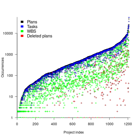
The average ratio of  is 8.4 (standard deviation 23). An exponential or power law (not Weibull) can be fitted to portions of the distribution of project sizes, measured in number of plans or tasks. If project size really does follow a single common distribution, a much larger sample size will be needed to reliably fit it.
The plot below shows, for each project (sorted by total person hours, in red), the number of elapsed days from start of first to end of last task (green), and number of people who worked on at least one task (blue) (projects implemented by a single person do not have consistent time data; code+data):
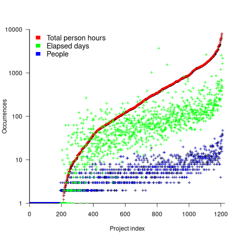
For a given number of person hours worked on a project, there is an order of magnitude variation in elapsed days and number of people who worked on at least one task.
This dataset contains a huge amount of detail, and I’m sure there are lots of patterns to be found. But, what are the important questions to ask, that would be useful to project managers. When I ask managers what project questions they would like answers, the response is often one of quizzical uncertainty. There are plenty of people promoting their opinions, and it’s very rare to encounter anybody asking meaningful questions.
Recent Comments