Archive
The fall of Rome and the ascendancy of ego and bluster
The idea that empirical software engineering started 10 years ago, driven by the availability of Open Source that could be measured, turns out to be a rather blinkered view of history.
A few months ago I was searching for a report and tried the Defense Technical Information Center (DTIC), which I had last tried many years ago. The search quickly located the report, plus lots of other stuff, and over the next few weeks I downloaded a few hundred interesting looking reports. These are pdfs that often don’t show up in Google searches and sometimes not on DTIC searches unless the right combination of words is used (many of the pdfs have been created by converting microfiche copies of the original paper, with some, often very good, OCR thrown into the mix).
It turns out that during the 1970s at the Rome Air Development Center (RADC was the primary research lab of the US Air Force) something of a golden age for empirical software engineering research occurred (compared to the following 25 years).
The ingredients necessary for great research came together at Rome during this decade: the US Department of Defense were spending huge amounts of money creating lots of software systems; the management at RADC understood the importance of measurement and analysis, and had the money to hire good consultants to do it.
Why did the volume of quality reports coming out of RADC decline in the 1980s (it closed in 1991)? I have no idea, perhaps the managers responsible for the great work moved on or priorities changed.
Ego and bluster is how software engineering research operated after the decline of Rome (I’m sure plenty of it occurred before and during Rome). A researcher or independent consultant had an idea about how they thought things worked (perhaps bolstered by a personal experience, not lots of data) and if their ego was big enough to think this idea was a good model of reality and they invest enough time blustering their way through workshop presentations and publishing papers, then the idea could become part of mainstream thinking in academia; no empirical evidence needed.
The start of the ego and bluster period could be said to be 1981, the year in which Software Engineering Economics by Barry Boehm was published, and 2008 as the end of the ego and bluster period (or at least the start of its decline) the year of publication of the 3rd edition of Applied Software Measurement by Capers Jones. Both books dress up tiny amounts of empirical data as ‘proof’ of the ideas being promoted.
Without measurement data researchers have to resort to bluster to hide the flimsy foundations of the claims being made, those with the biggest egos taking center stage. Commercial companies are loath to let outsiders measure what they are doing and very few measure what they are doing themselves (so even confidential data is rare). Most researchers moved onto other topics once they realised how little data was available or could be made available to them.
Around 2005, or so, the volume of papers using new empirical data started to grow and a trickle has now turned into a flood. Of course making use of empirical data does not prevent research papers being a complete waste of time and ego and bluster is still widely practiced (and not limited to software engineering).
While a variety of individuals and research groups around the world (sadly only individuals in the UK) are actively working on extracting and analysing open source systems, practical progress has been very slow. Researchers are still coming to grips with the basic characteristics of the data they are seeing.
The current legacy, in software engineering, of long standing beliefs (built on tiny datasets) is a big problem. Lots of researchers have not seen through the bluster and are spending lots of time and effort trying to accommodate the results they are obtaining with what are mistakenly taken to be ‘established’ theories. One example is “Program Evolution – Processes of Software Change” by Lehman and Belady, from the late 1970s. Researchers need to stop looking at Lehman’s ‘laws’ through rose tinted glasses; a modern paper making Lehman’s claims based on such a small set of measurements would be laughed.
Most of those now working with empirical data are students working towards a postgraduate degree, some of whom have gone on to get full-time research jobs. Unfortunately there are still many researchers applying the habits they acquired during the ego and bluster period; fit some old data using the latest fashionable technique, publish and quickly move on to the next fashionable technique. As Max Planck observed, science advances one funeral at a time.
What is the name should be given to this new period of software engineering research? We will probably have to wait many more years before things become clear.
Software Reliability is one report from the Rome period that is well worth checking out.
NASA sponsored research was hit and mostly miss. One very interesting sequence of experiments is documented in: Software reliability: Repetitive run experimentation and modeling and An experiment in software reliability.
Software Reliability: Lots of detailed data and thoughtful analysis
The 1978 book “Software Reliability” by Thayer, Lipow and Nelson is the only wide-ranging publicly available source of detailed software development project data that I am aware of. While analysis of Open Source, which started around 10 years ago, has added much more detail in some areas it has added almost nothing in other areas (e.g., manpower and requirements data). The analysis in this book is also very thorough, making good use of the statistical techniques available back in the day.
A few weeks ago I found an online pdf of the report from which the book is very closely derived. Anyone interested in software engineering should read this report, I’m not sure much of the state of the art has progressed that much since its publication in 1976.
The pdf was created from a microfiche copy of the original document and the numbers in some tables are illegible. I have photographed, in my copy of the book, the tables containing numbers printed using a small point size and you can download the jpegs (I don’t have the time to transcribe them to ascii text; please let me know if you do this).
Why did this book/report rapidly disappear into almost total obscurity? Perhaps it contained too much data and did too good a job of analysing it, compared to what came soon after it. Perhaps because it did not have a champion to sing its praises (wanting to build a personal career can have benefits for those other than the person doing the building).
COCOMO: Not worth serious attention
The Constructive Cost Model (COCOMO) was introduced to the world by the book “Software Engineering Economics” by Barry Boehm; this particular version of the model is now known by the year of publication, COCOMO 81. The book describes a model that estimates software project cost drivers, such as effort (in man months) and elapsed time; the data from the 63 projects used to help calibrate the equations appears on pages 496-497.
Only having 63 measurements to model such a complex problem means any predictions will have very wide error bounds; however, the small amount of data did not stop Boehm building an academic career out of over-fitting these 63 measurements using 17 input parameters (the COCOMO II book came out in 2000 and was initially calibrated by fitting 22 parameters to 83 measurement points and then by fitting 23 parameters to 161 measurement points; the measurement data does not appear to be publicly available).
A sentence on page 493 suggests that over-fitting may not be the only problem to be found in the data analysis: “The calibration and evaluation of COCOMO has not relied heavily on advanced statistical techniques.”
Let’s take the original data and duplicate the original analysis, before trying something more advanced (code+data).
A central plank of the COCOMO model is the equation:  , where
  is total effort in man months,
  a constant obtained by fitting the data,
  thousands of lines of source code and
  a constant obtained by fitting the data.
This post discusses fitting this equation for the three modes of software projects defined by Boehm (along with the equations he fitted):
- Organic, relatively small teams operating in a highly familiar environment:
 ,
, - Embedded, the product has to operate within strongly coupled, complex, hardware, software and operational procedures such as air traffic control:
 ,
, - Semidetached, an intermediate stage between the two extremes:
 .
.
The plot below shows kSLOC against Effort, with solid lines fitted using what I guess was Boehm’s approach and dashed lines showing fitted lines after removing outliers (Figure 6-5 in the book has the x/y axis switched; the points in the above plot appear to match those in this figure):
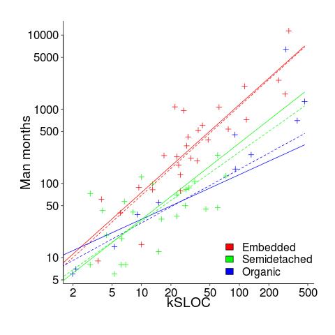
The fitted equations are (the standard error on the multiplier, , is around ±30%, while on the exponent, , the absolute value varies between ±0.1 and ±0.2):
- Organic:
 , after outlier removal
- Embedded:
 , after outlier removal
- Semidetached:
 , after outlier removal
  .
.
The only big difference is for Organic, which is very different. My first reaction on seeing this was to double check the values used against those in the book. How did Boehm make such a big mistake and why has nobody spotted it (or at least said anything) before now? Papers by Boehm’s students do use fancy statistical techniques and contain lots of tables of numbers relating to COCOMO 81, but no mention of what model they actually found to be a good fit.
The table on pages 496-497 contains man month estimates made using Boehm’s equations (the EST column). The values listed are a close match to the values I calculated using Boehm’s Semidetached equation, but there are many large discrepancies between printed values and values I calculated (using Boehm’s equations) for Organic and Embedded. If the data in this table contains a lot of mistakes, it may explain why I get very different values fitting the data for Organic. Some ther columns contain values calculated using the listed EST values and the few I have checked are correct, so if there was an error in the EST value calculation it must have occurred early in the chain of calculations.
The data for each of the three modes of software development contain several in your face outliers (assuming the values are correct). Based on the fitted equations is does not look like Boehm removed these (perhaps detecting outliers is an advanced technique).
Once the very obvious outliers are removed the quadratic equation,  , becomes a viable competing model. Unfortunately we don’t have enough data to do a serious comparison of this equation against the COCOMO equation.
In practice the COCOMO 81 model has been found to be highly inaccurate and very much dependent upon the interpretation of the input parameters.
Further down on page 493 we have: “I have become convinced that the software field is currently too primitive, and cost driver interaction too complex, for standard statistical techniques to make much headway;”.
With so much complexity and uncertainty, careful application of statistical techniques is the only way of reliable way of distinguishing any signal from noise.
COCOMO does not deserve anymore serious attention (the code+data includes some attempts to build alternative models, before I decided it was not worth the effort).
Applied Software Measurement: shame about the made up numbers
“Applied Software Measurement” by Capers Jones (no relation) is widely cited, but I find it a very frustrating book; while the text is full of useful commentary the numbers in the tables are mostly made up or estimated from other numbers (some of which may be actual measurements).
This book’s many tables of numbers will catch the attention of anyone searching for software engineering data (which until recently was very hard to find). However, closer inspection of the numbers suggests that the real purpose of the empirical looking tables is to serve as eye-candy to impress casual readers.
Let’s take as an example the analysis of multiple implementations, in different languages, of software implementing telephone switching system functionality. The numbers are from the third edition of the book (the one I have; code+data, separate paper discussing the numbers).
Below are the numbers from Table 2-7: Function Point and Source Code Sizes for 10 Versions of the Same Project.
All those 1,500’s are a bit suspicious; the second paragraph under the table says “… the original sizes ranged from about 1,300 to 1,750 …”. Why has a gratuitous 1.5% error been introduced?
Where did the values for language level come from? I once wrote the semantics phase of a CHILL compiler in Pascal and would have put CHILL’s language level on a par with Ada83. Objective C at 11 is surely a joke. Language level is a number, so obviously we can take its average.
This table looks like it has one column of actual data. Oh, five pages before the table appears we are told that the Ada95 and Objective C results were modeled, i.e., made up. So there are really only eight real implementations, not ten.
Language Function pts Language level LOC/Func. Pt. Size in LOC Assembly 1,500 1 250 375,000 C 1,500 3 127 190,500 CHILL 1,500 3 105 157,500 PASCAL 1,500 4 91 136,500 PL/I 1,500 4 80 120,000 Ada83 1,500 5 71 106,500 C++ 1,500 6 55 82,500 Ada95 1,500 7 49 73,500 Objective C 1,500 11 29 43,500 Smalltalk 1,500 15 21 31,500 Average 1,500 6 88 131,700 |
Moving on to Table 2-6, see below: “Staff Months of Effort for 10 Versions of the Same Software Project”
The use of two decimal places of accuracy is an obvious red flag for wanting to impress via appearance of accuracy.
Is the requirements effort based on one known value, or is it estimated? Why the jump in design time when we get to C++? Does management time really have such a strong dependency on language used?
Language Require.. Design Code Test Document Management TOTAL Effort Assembly 13.64 60.00 300.00 277.78 40.54 89.95 781.91 C 13.64 60.00 152.40 141.11 40.54 53.00 460.69 CHILL 13.64 60.00 116.67 116.67 40.54 45.18 392.69 PASCAL 13.64 60.00 101.11 101.11 40.54 41.13 357.53 PL/I 13.64 60.00 88.89 88.89 40.54 37.95 329.91 Ada83 13.64 60.00 76.07 78.89 40.54 34.99 304.13 C++ 13.64 68.18 66.00 71.74 40.54 33.81 293.91 Ada95 13.64 68.18 52.50 63.91 40.54 31.04 269.81 Objective C 13.64 68.18 31.07 37.83 40.54 24.86 216.12 Smalltalk 13.64 68.18 22.50 27.39 40.54 22.39 194.64 |
The above table makes more sense when LOC is plotted against Total Effort (in man months), see below:
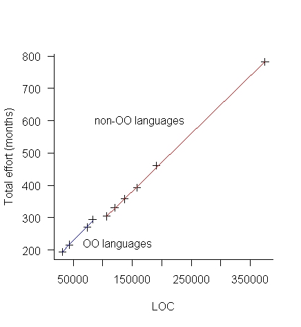
The blue line is for the object oriented languages (i.e., the last four rows of the table) and the red line everything else. Those two straight lines fit the data so well; I think that Total Effort was calculated from LOC and various rules of thumb used to create percentages for requirements, design, code, test, documentation and management.
There is no new data in the above table, it was all calculated from LOC and informed arm waving.
Table 2-9 and Table 2-11 list Total Effort (which has been estimated from LOC) and columns of values created by dividing or multiplying this by other estimated values.
Table 2-12, see below: “Defect Potentials for 10 Versions of the Same Software Project”
What is a Defect Potentials?
Again, a sudden jump in the design numbers at C++.
Language Require.. Design Code Document Bad Fix TOTAL Defects Assembly 1,500 1,875 7,500 900 1,060 12,835 C 1,500 1,875 3,810 900 728 8,813 CHILL 1,500 1,875 3,150 900 668 8,093 PASCAL 1,500 1,875 2,730 900 630 7,635 PL/I 1,500 1,875 2,400 900 601 7,276 Ada83 1,500 1,875 2,130 900 576 6,981 C++ 1,500 2,025 1,650 900 547 6,622 Ada95 1,500 2,025 1,470 900 531 6,426 Objective C 1,500 2,025 870 900 477 5,772 Smalltalk 1,500 2,025 630 900 455 5,510 |
Plotting total defects against LOC (below) suggests that “Defect Potentials” is a number calculated from LOC, i.e., no connection with actual defects found.
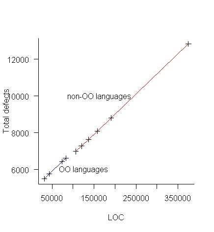
Table 2-13 lists Total Defects (which has been estimated from LOC) and columns of values created by dividing or multiplying this by other estimated values.
So the book contains six impressive looking tables whose numbers have been calculated in one way or another from lines of code. A very good description of the many other tables in the book.
Survival time of Linux distributions
Creating and maintaining Linux distributions is a surprisingly popular activity. The GNU/Linux Distribution Timeline listed over 500 distributions by the time recording stopped at the end of 2012.
Once a distribution becomes available, how long do the people involved on a distribution continue to maintain it? The plot below shows the survival curve for Linux distributions based on their original parent distribution; the five most popular parent distributions are shown (code+data).
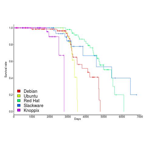
The plus-signs on lines are censored data, that is distributions that are still actively maintained (or at least not listed as no longer supported) when maintenance work on the timeline stopped (October 2012).
My interpretation of the data is that when the maintainers of a parent distribution are responsive to community pressure, it is difficult to motivate people to maintain a distribution derived from it.
RedHat is a commercial distribution and likely to be less focused on the developer community.
Ubuntu (79 derived distributions) and Knoppix (20 derived distributions) are relative newcomers. It looks like Knoppix has been squeezed out by the top 4.
Update in 2024
Fabio Loli has been updating the timeline.
Recent Comments