Archive
Who are the famous academics in software engineering?
Who are today’s ‘famous’ academics in software engineering?
Famous as in, you can mention their name when chatting with general software developers, and expect those present to have heard of them, or you have heard their names dropped into a conversation, say, at least 3+ times this year (I’m excluding academics who are famous within one specific niche of software engineering). Academic, as in, works in an institution of secondary or tertiary higher learning.
When I started out in industry, the works of Knuth and Dijkstra were cited (not always accurately), people would talk about Ted Codd’s latest position on how best to structure a database. Tony Hoare later became known through his books, and Leslie Lamport for distributed systems and perhaps LaTeX. In very large niches, William Kahan for numerical analysis, and Barbara Liskov for the Liskov substitution principle.
Anyone suggesting Kernighan and Ritchie, of C and Unix fame, is overlooking the fact they worked in an industrial research lab.
A book series continues to maintain Knuth’s fame, while Dijkstra kept himself in the news by being a source of controversial quotes for industry journalists, and for kicking off the Go-To statement considered harmful debate (the latter is likely the reason that anybody has heard of him today). Has Kahan escaped his niche, even though use of floating-point arithmetic is now perhaps even more niche than it used to be?
How might academics become famous?
Widely used algorithms/metrics/techniques named after a person generates a kind of anonymous name recognition. For instance, Halstead complexity metric and McCabe’s cyclomatic complexity metric, and from the 1990s Shor’s algorithm.
Some people achieve fame through their association with a language. Academic name/language pairs include: McCarthy/Lisp, Wirth/Pascal, Stroustrup/C++ (worked in industry, university, industry, university), Peyton Jones/Haskell (university, industrial research, industry), Leroy/OCaml, Meyer/Eiffel.
An influential book, or widely read blog can generate a kind of fame.
Many academics have written an ‘algorithms’ book, and readers may have fond memories of the particular book they used as an undergraduate. Barry Boehm wrote “Software Engineering Economics”, but is more likely to be known for the model he spent his life promoting, i.e., the COCOMO model.
Fred Brooks, author of one of the most famous books in software engineering The Mythical Man Month, was not an academic worked in industry and then academia.
I have always been surprised by how many Turing award winners I have never heard of, or while recognizing a name am completely unfamiliar with their work. I am less surprised by my failure to recognise around half the names in the Wikipedia category software engineering researchers.
A few people are known because of the widespread use of their software (Linus Torvalds has never been an academic). Richard Stallman, employed as an academic, originally became famous as the author of the GNU version of emacs and gcc; the fame from the Free Software Foundation came after copyleft took off.
Are there academics who have become ‘famous’ in software engineering this century? I’m not in a position to answer this because I don’t read introductory software books, and generally avoid bike-shed discussions.
Does the resurgence of interest in AI mean that Judea Pearl’s fame is no longer niche?
I do read recent academic papers, and the only person on the list of most frequently cited authors in my evidence-based software engineering book with any claim to fame, researches cognitive neuroscience, i.e., Stanislas Dehaene.
Is software engineering a field where it is possible for a person, academic or otherwise, to become famous?
If there are fame worthy discoveries waiting to be made, or fame worthy software engineering book waiting to be written, how likely is it that the people responsible will be academics? A lot of the advances in software engineering have been made and continue to be made by those working in industry.
Suggestions relating to (in)famous academics welcome.
Benchmarking fuzzers
Fuzzing has become a popular area of research in the reliability & testing community, with a stream of papers claiming to have created a better tool/algorithm. The claims of ‘betterness’, made by the authors, often derive from the number of previously unreported faults discovered in some collection of widely used programs.
Developers in industry will be interested in using fuzzing if it provides a cost-effective means of discovering coding mistakes that are likely to result in customers experiencing a serious fault. This requirement roughly translates to: minimal cost for finding maximal distinct mistakes (finding the same mistake more than once is wasted effort); whether a particular coding mistake is likely to produce a serious customer fault is a decision decided by people.
How do different fuzzing tools compare, when benchmarking the number of distinct mistakes they each find, for a given amount of cpu time?
TL;DR: I don’t know, and this approach is probably not a useful way of comparing fuzzers.
Fuzzing researchers are currently competing on the number of previously unreported faults discovered, i.e., not listed in the fuzzed program’s database of fault reports. Most research papers only report the number of distinct faults discovered in each program fuzzed, the amount of wall clock hours/days used (sometimes weeks), and the characteristics of the computer/cluster on which the campaign was run. This may be enough information to estimate an upper bound on faults per unit of cpu time; more detailed data is rarely available (I have emailed the authors of around a dozen papers asking for more detailed data).
A benchmark based on comparing faults discovered per unit of cpu time only makes sense when the new fault discovery rate is roughly constant. Experience shows that discovery time can vary by orders of magnitude.
Code coverage is a fuzzer performance metric that is starting to be widely used by researchers. Measures of coverage include: statements/basic blocks, conditions, or some object code metric. Coverage has the advantage of providing defined fuzzer objectives (e.g., generate input that causes uncovered code to be executed), and is independent of the number of coding mistakes present in the code.
How is a fuzzer likely to be used in industry?
The fuzzing process may be incremental, discovering a few coding mistakes, fixing them, rinse and repeat; or, perhaps fuzzing is run in a batch over, say, a weekend when the test machine is available.
The current research approach is batch based, not fixing any of the faults discovered (earlier researchers fixed faults).
Not fixing discovered faults means that underlying coding mistakes may be repeatedly encountered, which wastes cpu time because many fuzzers terminate the run when the program they are testing crashes (a program crash is a commonly encountered fuzzing fault experience). The plot below shows the number of occurrences of the same underlying coding mistake, when running eight fuzzers on the program JasPer; 77 distinct coding mistakes were discovered, with three fuzzers run over 3,000 times, four run over 1,500 times, and one run 62 times (see Green Fuzzing: A Saturation-based Stopping Criterion using Vulnerability Prediction by Lipp, Elsner, Kacianka, Pretschner, Böhme, and Banescu; code+data):
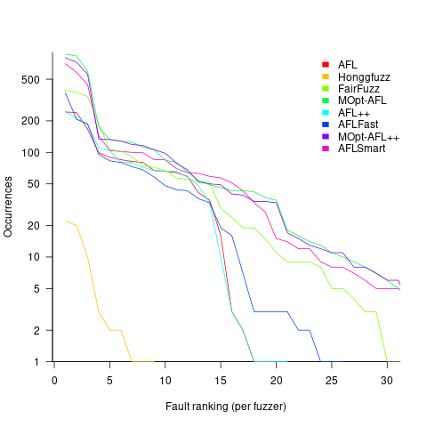
I have not seen any paper where the researchers attempt to reduce the number of times the same root cause coding mistake is discovered. Researchers are focused on discovering unreported faults; and with around 98% of fault discoveries being duplicates, appear to have resources to squander.
If developers primarily use a find/fix iterative process, then duplicate discoveries will be an annoying drag on cpu time. However, duplicate discoveries are going to make it difficult to effectively benchmark fuzzers.
Research ideas for 2023/2024
Students sometimes ask me for suggestions of interesting research problems in software engineering. A summary of my two recurring suggestions, for this year, appears below; 2016/2017 and 2019/2020 versions.
How many active users does a program or application have?
The greater the number of users, the greater the number of reported faults. Estimates of program reliability have to include volume of usage as an integral part of the calculation.
Non-trivial amounts of public data on program usage is non-existent (in a few commercial environments, users are charged for using software on a per-usage basis, but this data is confidential). Usage has to be estimated by indirect means.
A popular indirect technique for estimating the popularity of Github repos is to count the number of stars it has; however, stars have a variety of interpretations. The extent to which Github stars tracks usage of the repo’s software is not known.
Other indirect techniques include: web server logs, installs of the application, or the operating system.
One technique that has not yet been researched is to make use of the identity of those reporting faults. A parallel can be drawn with the fish population in lakes, which is not directly visible. Ecologists have developed techniques for indirectly estimating the population size of distinct creatures using information about a subset of the population, and some of the population models developed for ecology can be adapted to estimating program user populations.
Estimates of population size can be obtained by plugging information on the number of different people reporting faults, and the number of reports from the same person into these models. This approach is not as easy as it sounds because sometimes the same person has multiple identities, reported faults also need to be deduplicated and cleaned (30-40% of reports have been found to be requests for enhancements).
Nested if-statement execution
As if-statement nesting depth increases, the number of conditions controlling the execution of the enclosed code increases.
Being able to estimate the likelihood of executing the code controlled by an if-statement is of interest to: compilers wanting to target optimizations along the most frequently executed paths, special handling for error paths, testing along the least/most likely paths (e.g., fuzzers wanting to know the conditions needed to reach a given block), those wanting to organize code for ease of understanding, by reducing cognitive effort to understand.
Possible techniques for analysing the likelihood of executing code controlled by one or more nested if-statements include:
- Compiler writers have discovered various heuristics for predicting the likely outcome of a branch, and there are probably more to be discovered. Statement coverage counts provides a ground truth against which to compare ideas,
- analysis of the conditional expression,
- mathematical analysis of the distribution of values of variables in conditional expressions.
The lifetime of performance coding issues
Coding activities that a developer might spend time on include: adding new functionality, fixing a reported fault, or fiddling with existing code with the intent of making it ‘better’ in some sense (which these days goes by the catch-all name of refactoring).
Improving performance, e.g., changing software to use less cpu/memory is considered, by developers, to make it ‘better’ (whether users are likely to notice the difference, or management see a ROI is for another article). There is a breed of developer whose DNA encodes for pleasure receptors that are only fire when working to reduce the amount of cpu/memory used by a program.
The paper Characterizing the evolution of statically-detectable performance issues of Android Apps by Das, Di Penta, and Malavolta studied the creation/removal of nine distinct performance coding issues in the source of 316 Android Apps (118 Apps contained five or more issues); a total of 2,408 performance issues were tracked.
What patterns might be present in the paper’s performance issues data?
I would expect there to be more creations in Apps containing more code, and more removals the longer an App is maintained; both very obvious. With more developers working on an App, there are going to be more creations and removals; do they cancel out? Management might decide to invest time in performance improvements for the next release, which would cause a spike in the number of removals per unit time.
How long do the nine performance issues survive in code, before being removed? The plot below shows the Kaplan Meier survival curve for Apps containing at least five issues (dotted blue/green are the 95% confidence intervals, code+data):
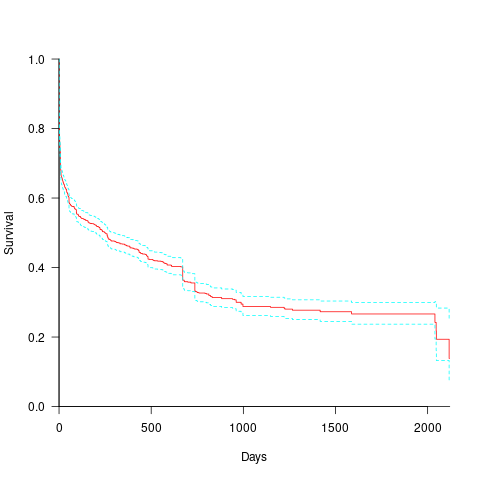
Around 15% of issues were removed on the day they are created, and by the eighth day around 30% had been removed. The roughly steady decline lasts for two-years, followed by almost stasis. Is two-years the active development lifetime of a successful Android App?
In isolation, the slope of the survival curve between eight days and two-years is not that interesting (it could be used to rule out models of the issue discovery process, e.g., happenstance discovery while working on other tasks). However, comparing it against the corresponding survival curve for reported faults tells us something about developer/management investment priorities for the two kinds of tasks, as measured by time to fix (which is a proxy for effort invested).
Unfortunately, this study did not collect information on coding mistake lifetimes, or time between a fault being reported and fixed. There have been studies investigating the survival time of coding mistakes. Reported faults should have the lowest survival rate, while the survival of coding mistakes will depend on the number of users (i.e., more users creates more opportunities to experience a fault and report it).
What factors influence performance issue time-to-fix?
The data includes information on the kind of performance issue, the number of times the App has been downloaded from the Google Play Store, and the number of contributors to the App.
Using these variables, a Cox proportional hazards model was fitted to model the survival time. In a proportional hazards model, the model coefficients are not absolute values, but provide ratio information. For instance, the following table shows the coefficients of the fitted model (code+data). Using these coefficients, we can compare the time taken to fix, say, a FloatMath issue relative to a ViewTag issue. The coefficient ratio  is the estimated ratio of fix times of the two respective issues.
Coefficient Standard error Performance issue FloatMath 0.64445 0.14175 HandlerLeak 0.69958 0.12736 Recycle 0.83041 0.11386 UseSparseArrays 0.73471 0.12493 UseValueOf 0.64263 0.11827 ViewHolder 0.87253 0.14951 ViewTag 5.24257 0.46500 Wakelock 3.34665 0.72014 Downloads 50-100 0.62490 0.26245 100-500 0.64699 0.22494 500-1000 0.56768 0.23505 1000-5000 0.50707 0.22225 5000-10000 0.53432 0.22486 10000-50000 0.62449 0.21626 50000-100000 0.42214 0.23402 100000-500000 0.21479 0.25358 1000000-5000000 0.40593 0.21851 10000000-50000000 0.03474 0.61827 100000000-500000000 0.30693 0.39868 1000000000-5000000000 0.41522 0.61599 NA 0.03868 1.02076 Contributors 1.04996 0.01265 |
There is not a lot of difference in the coefficients for the number of downloads (the model fit is poor when the Standard error is close to the Coefficient value).
The paper Investigating Types and Survivability of Performance Bugs in Mobile Apps analyses a smaller dataset of performance issue lifetimes.
Predicting the size of the Linux kernel binary
How big is the binary for the Linux kernel? Depending on the value of around 15,000 configuration options, the size of the version 5.8 binary could be anywhere between 7.3Mb and 2,134 Mb.
Who is interested in the size of the Linux kernel binary?
We are not in the early 1980s, when memory for a desktop microcomputer often topped out at 64K, and software was distributed on 360K floppies (720K when double density arrived; my companies first product was a code optimizer which reduced program size by around 10%).
While desktop systems usually have oodles of memory (disk and RAM), developers targeting embedded systems seek to reduce costs by minimizing storage requirements, security conscious organizations want to minimise the attack surface of the programs they run, and performance critical systems might want a kernel that fits within a processors’ L2/L3 cache.
When management want to maximise the functionality supported by a kernel within given hardware resource constraints, somebody gets the job of building kernels supporting various functionality to find out the size of the binaries.
At around 4+ minutes per kernel build, it’s going to take a lot of time (or cloud costs) to compare lots of options.
The paper Transfer Learning Across Variants and Versions: The Case of Linux Kernel Size by Martin, Acher, Pereira, Lesoil, Jézéquel, and Khelladi describes an attempt to build a predictive model for the size of the kernel binary. This paper includes an extensive list of references.
The author’s approach was to first obtain lots of kernel binary sizes by building lots of kernels using random permutations of on/off options (only on/off options were changed). Seven kernel versions between 4.13 and 5.8 were used, producing 243,323 size/option setting combinations (complete dataset). This data was used to train a machine learning model.
The accuracy of the predictions made by models trained on a single kernel version were accurate within that kernel version, but the accuracy of single version trained models dropped dramatically when used to predict the binary size of later kernel versions, e.g., a model trained on 4.13 had an accuracy of 5% MAPE predicting 4.13, when predicting 4.15 the accuracy is 20%, and 32% accurate predicting 5.7.
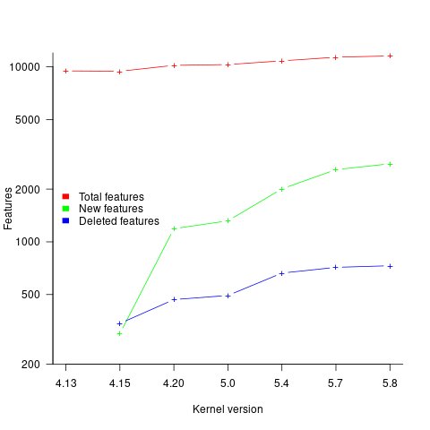
I think that the authors’ attempt to use this data to build a model that is accurate across versions is doomed to failure. The rate of change of kernel features (whose conditional compilation is supported by one or more build options) supported by Linux is too high to be accurately modelled based purely on information of past binary sizes/options. The plot below shows the total number of features, newly added, and deleted features in the modelled version of the kernel (code+data):
What is the range of impacts of each build option, on binary size?
If each build option is independent of the others (around 44% of conditional compilation directives in the kernel source contain one option), then the fitted coefficients of a simple regression model gives the build size increment when the corresponding option is enabled. After several cpu hours, the 92,562 builds involving 9,469 options in the version 4.13 build data were fitted. The plot below shows a sorted list of the size contribution of each option; the model  is 0.72, i.e., quite a good fit (code+data):

While the mean size increment for an enabled option is 75K, around 40% of enabled options decreases the size of the kernel binary. Modelling pairs of options (around 38% of conditional compilation directives in the kernel source contain two options) will have some impact on the pattern of behavior seen in the plot, but given the quality of the current model ( is 0.72) the change is unlikely to be dramatic. However, the simplistic approach of regression fitting the 90 million pairs of option interactions is not practical.
What might be a practical way of estimating binary size for any kernel version?
The size of a binary is essentially the quantity of code+static data it contains.
An estimate of the quantity of conditionally compiled source code dependent on a given option is likely to be a good proxy for that option’s incremental impact on binary size.
It’s trivial to scan source code for occurrences of options in conditional compilation directives, and with a bit more work, the number of lines controlled by the directive can be counted.
There has been a lot of evidence-based research on software product lines, and feature macros in particular. I was expecting to find a dataset listing the amount of code controlled by build options in Linux, but the data I can find does not measure Linux.
The Martin et al. build data is perfectfor creating a model linking quantity of conditionally compiled source code to change of binary size.
Recent Comments