Archive
Readability of anonymous inner classes and lambda expressions
The available evidence on readability is virtually non-existent, mostly consisting of a handful of meaningless experiments.
Every now and again somebody runs an experiment comparing the readability of X and Y. All being well, this produces a concrete result that can be published. I think that it would be a much more effective use of resources to run eye tracking experiments to build models of how people read code, but then I’m not on the publish or perish treadmill.
One such experimental comparison of X and Y is the paper Two N-of-1 self-trials on readability differences between anonymous inner classes (AICs) and lambda expressions (LEs) on Java code snippets by Stefan Hanenberg (who ran some experiments on the benefits of strong typing) and Nils Mehlhorn.
How might the readability of X and Y be compared (e.g., Java anonymous inner classes and lambda expressions)?
If the experimenter has the luxury of lots of subjects, then half of the subjects can be assigned to use X and half to use Y. When only a few subjects are available, perhaps as few as one, an N-of-1 experimental design can be used.
This particular study is worth discussing because it appears to be thought out and well run, as well as illustrating the issues involved in running such experiments, not because the readability of the two constructs is of particular interest. I think that developer choice of anonymous inner classes or lambda expressions is based on fashion and/or habit, and developers will claim the construct they use is the most readable one for them.
The Hanenberg and Mehlhorn study involved two experiments, using a N-of-1 design. In the first experiment task, subjects saw a snippet of code and had to count the number of parameters in either the anonymous inner class or the lambda expression (whose parameters were either untyped or typed); in the second experiment task subjects had to count the number of defined parameters that were used in the body of the anonymous inner class or lambda expression. English words were used for parameter names.
Each of the eight subjects saw the same set of randomly shuffled distinct 600 code snippets. The time taken to answer and correct/incorrect answer status were recorded. The snippets varied in the number of parameters and kind of construct; for task 1: 0-4 parameters, 3-kinds of construct, repeated 40 times, giving  distinct snippets; for task 2: 0-3 parameters used out of 3 parameters, 3-kinds of construct, repeated 50 times, giving
  distinct snippets.
The first task requires subjects to locate the definition of the construct, count the number of parameters, and report the count. The obvious model is different constructs require different amounts of time to locate, and that each parameter adds a fixed amount to the response time; there may be a small learning component.
Fitting a simple regression model shows (depending on choice of outlier bounds) that averaged over all subjects each parameter increased response time by around 80 msec, and that response was faster for lambda expressions (around 200 msec without parameter types, 90 msec if types are present); code+data. However, the variation across subjects had a standard deviation that was similar to these means.
The second task required subjects to read the body of the code, to find out which parameters were used. The mean response time increased from 1.5 to 3.7 seconds.
I was not sure whether to expect response time to increase or decrease as the number of parameters used in the body of the code increased (when the actual number of parameters is always three).
A simple fitted regression model finds that increase/decrease behavior varies between subjects (around 50 msec per parameter used); code+data. I am guessing that performance behavior depends on the mental model used to hold the used/not yet used information.
The magnitude of the performance differences found in this study mimics that seen in most human based software engineering experiments, that is, the impact of the studied construct is very small.
Local variable naming: some previously unexplored factors
Naming is a complicated topic, with factors including the semantic associations triggered by a name in the developer’s mind (e.g., arithmetic or bitwise operand), visual similarity to other identifiers, and usability (e.g., fewer characters).
Within a method, local variables coexist with other local variables that are visible over some number of lines of code.
Does the size of a method, in lines of code, or number of local variables have an impact on the names chosen (e.g., does the need to think up many different names affect the length of the name chosen)?
The paper A Large-Scale Investigation of Local Variable Names in Java Programs: Is Longer Name Better for Broader Scope Variable? appears to address this question, but the paper is not freely available (although its data is available). I learned about it, and its data, while reading another paper: Reanalysis of Empirical Data on Java Local Variables with Narrow and Broad Scope by Dror Feitelson.
The data was extracted from 1,000 popular Java projects, whose 46,283 files contained 637,077 local variables. The collected information includes: source filename, name, line variable defined, and line last used. Additional columns include the number of characters in the name, and a classification of the components of the name (e.g., dictionary word, abbreviation, number).
For the following analysis, I mapped each variable to a most likely associated method by coalescing overlapping variable defined/last-used ranges. A total of 204,503 methods were formed.
To analyse the impact of other local variables and method size on naming, we first need some information on the number of local variables defined in Java methods, and the number of lines contained in Java methods.
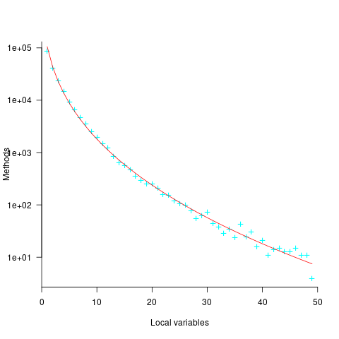
Approximately 50% of Java methods define five or fewer local variables. The plot below shows the number of Java methods defining a given number of local variables; the fitted regression equation, red line, has the form  , where
  is the number of local variables (code+data):
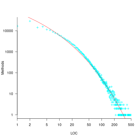
The reason most method define few local variables is that most methods only contain a few lines. The plot below shows the number of Java methods containing an estimated number of lines of code; the fitted regression equation, red line, has the form  , where
  is estimated lines of code (code+data):
The plot below shows the number of local variables against estimated lines of code in the corresponding method; the fitted regression equation, red line, has the form  , where is the number of local variables (code+data):
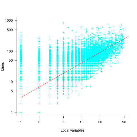
The strong connection between the number of lines of code and number of local variables in a method means that these two factors are effectively interchangeable in a regression model.
A local variable name is likely to be chosen before all, or even any, of the code that uses it is written. The hypothesis that the choice of a variable name is influenced by the length of a method, or the span of lines over which the variable is used, assumes some degree of foresight on the part of the developer.
The cited papers posed the question at the start of this post, and I built a variety of regression models looking to find those factors that are the best predictors of the length of the name (measured in characters or number of subcomponents), or the extent to which the length of the name predicted the amount of code over which it was used (either as a percentage or actual number of lines). Factors used include: order of variable definition in function, percentage of method code over which variable was used. See code+data.
The better models explained up to around 5% of the variance in the data. So there is an effect, but it’s very small. For instance, the model , where
  is the number of lines between variable definition and its last use, and
  is the number of characters in its name, is effectively a relationship between the mean value of these two factors that captures some of the variance around their means.
Motivation and software development
If people were not motivated to write software, computers would not have anything to do. What motivates a person to write software?
The source of human motivation may be intrinsic, as when pleasure is derived from performing the activity, or it may be extrinsic, such as being paid.
For some developers, writing software is a hedonistic activity. Intrinsic motivation continues to be the attractive force behind very many Open source projects.
People have to make a living, and being paid to write software creates an extrinsic motivation.
What do we know about human motivation?
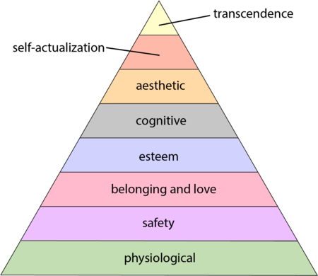
The 1943 paper A Theory of Human Motivation introduced Maslow’s hierarchy of needs, which is now often used as a structure for thinking about motivation. The image below, from Wikipedia, shows Maslow’s hierarchy:
Managers have long known that various kinds of carrots & sticks can be used to incentivize people to behave in a particular way, i.e., applying extrinsic motivation.
Incentives are actively researched in business and marketing departments. Unfortunately, sometimes more fashionable topics, such as cognitive biases, divert researcher’s interest.
Despite its fundamental importance, developer motivation is rarely considered, let alone a subject of research, within computing departments.
As purveyors of intangible goods, the software industry is aware of many issues around motivation. Managers of software teams appreciate the impact of team motivation on performance. Team motivation is a perennial topic of discussion for the Agile coaches and Scrum masters I meet. Companies selling products offering an API hire developer evangelists, whose job is to motivate third-party developers to use this API.
Software systems that continue to be used become part of the fabric of larger, more complex, systems. The motivations of the inhabitants of complex systems can have many unintended consequences.
Motivation is an intangible that cannot be measured directly; its effect has to be inferred from the results produced by the behaviors it drives. Distinguishing between two diametrically different motivations can present a conundrum, e.g., distinguishing between developers following Parkinson’s law or striving to meet a deadline.
Books don’t usually have much to say about the human side of software product management. A well-known exception is Peopleware: Productive Projects and Teams.
My evidence-based software engineering book should have had a chapter devoted to motivation, but given its focus on publicly available data, I had to make do with several 1-page subsections.
Accuracy of Function Point estimates
The number of Function points, FP, contained in the implementation of a software system are counted by following a specified counting process. The number of FP counted for a project is mapped to a cost estimate by multiplying the number of FP by the predetermined cost value of one FP; the predetermined value is based on cost data from similar previous projects within the company. The FP process is so popular as a unit of cost estimation that there are six different ISO standards specifying six different Function point measurement processes.
TL;DR: Estimated cost is not as accurate as traditional time based estimating, although the estimation process may produce consistent FP counts.
The FP certification schemes run by various organizations require applicants to pass exams that check they are consistently following the specified processes to produce consistent FP counts, i.e., that certified practitioners give very similar answers for the same implementation problem. Experiments where subjects used different counting processes to count FP for the same task, have found what looks like a linear relationship between various pairs of FP counting processes.
Having certified FP employees/consultants produce similar counts is all well and good, but what management actually wants is a close correspondence between estimated and actual costs. What does the available data show with regard to FP cost estimation accuracy?
I know of two FP/Cost datasets, one containing 149 points from one company (actual costs have been normalised), and the other 492 points from three companies (actual costs in Euros; FP used is IFPUG); this dataset also includes additional context information and is used in this post’s analysis.
What is the relationship between an estimate based on FP and actual cost? The plot below show FP against actual cost, the red line is the fitted regression equation  , the grey line shows
  (code+data):
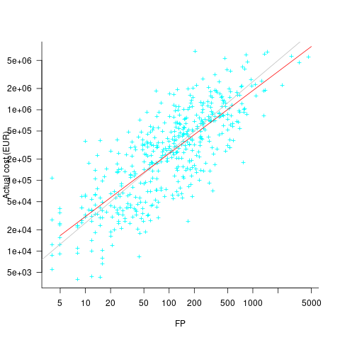
The power law exponent, 0.8, is slightly smaller than the 0.85 value found when fitting time estimates to actual times.
The dataset includes information specifying: anonymous organization ID, development method (78.5% plan driven and 21.5% Scrum), business domain (e.g., Call center, Mortgages, Front office), and various 0/1 flags each denoting a particular characteristic.
Including this information in a regression model finds that some of them have an impact on the FP to actual cost mapping. This is not surprising, since the FP/cost mapping is intended to be based on similar previous projects. The fitted model has the form:

where:  ,
,  ,
,  , and
, and  are constants for the corresponding items from the fitted regression model.
The fitted value for the scrum the development method is  , and
, and  for plan based (i.e., waterfall), i.e., Agile FP are cheaper than Waterfall FP. The idea of using both FP and scrum had not crossed my mind. Estimating via FP requires a detailed breakdown of the work to be done, while scrum is a process that discovers the work to be done. Perhaps a scrum like methodology was used to implement the detailed breakdown used to count FPs. The apparent lower cost of scrum FPs could just be a result of discovering that some planned functionality was not required.
How accurate were the FP estimates?
It is not possible to answer this question between we don’t know the cost assigned to one FP; in the above plot, the grey lines shows  .
.
We can calculate an estimate accuracy relative to the fitted model (the red line above). The mapping from FP to cost can vary between organizations, and the following analysis is based on the data for each distinct organization. The plot below shows the points, and associated fitted regression line, for the three organizations (code+data):
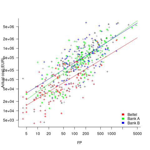
Each organization’s fitted regression model can be used to calculate confidence intervals. Approximately 68% of FP estimates could be off by over a factor two (between 2.3 and 2.5) from the mean actual cost, while for the 95% interval FP estimates could be off by over a factor five (it varied between 5.0 and 5.8); code+data. The corresponding factors for traditional developer time estimation are two and four.
The exponent varies between 0.72 and 0.84, with Beltel and Bank B having very similar values (the exponent for time estimates is often close to 0.85). The FP/Cost mapping is likely to be similar for the two banks, but lower for the telecoms company.
Does slicing the data by organization and business domain reduce the width of the confidence intervals, i.e., smaller multiplication factor? In some cases the width is reduced, but in other cases the width is increased; the 68% factor is between 1.9 and 3.1, the 95% factor is between 3.2 and 9.4.
Recent Comments