Archive
Answering via a scale to improve estimation accuracy
The human brain differs from the brain of other animals in having two number processing systems: 1) the approximate number system (present in other animals), and 2) language.
Round numbers are often given in answers when using language, to questions having a numeric answer. While use of round numbers may be conversationally appropriate, they decrease the accuracy of the answer.
Numeric values can be specified without using language. For instance, by pointing at a position on a scale representing a sequence of increasing/decreasing values, such as a ruler. Are answers given by pointing at a scale less likely to be round numbers, and more importantly are they likely to be more accurate than answers given using language?
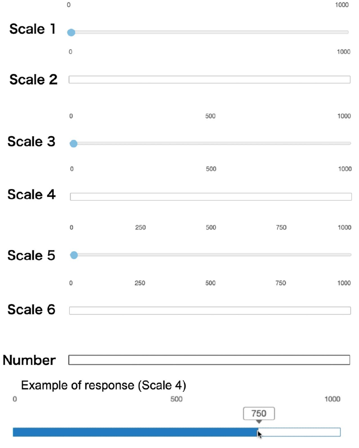
Various studies by psychologists have investigated response differences between answering using language and scales. The analysis below is based on data from the paper: On the round number bias and wisdom of crowds in different response formats for numerical estimation by Honda, Kagawa and Shirasuna. This study asked 1,805 subjects to estimate the number of dots in an image, like the one below, with images containing: 183, 287, 360, 453, 554, 633, 719, 807, or 986 dots (randomly selected):

Subjects responded using a randomly selected one of six different scales or using language (i.e., typing a number). The scales differed in axis labeling and some were zero based (subjects had to slide the blue colored circle from zero to a position, rather than clicking on a position); see image below:
The plot below shows the normalised occurrences of estimate values (rounded to the nearest value divisible by five) made using language (red) and one of the scales (blue/green), with grey line showing actual number of dots. There was little difference between the various kinds of scales, and all the scale answers have been aggregated (code+data):
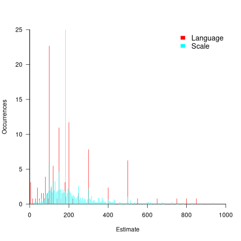
The red spikes clearly show many language given answers are at round numbers. The answers given using a scale are much less likely to be round numbers, with the blue/green lines showing the use of a wider selection of estimates.
Are answers given using language likely to be more or less accurate than answer given using a scale?
The plot above shows that few responses are close to the actual value, which means that no fitted model is going to explain much of the variability in the data. All the regression models I fitted to the difference between answers and actuals found that languages responses were less accurate, on average (code+data). Combining the explanatory variables in a variety of different ways did not significantly affect the quality of the fitted model.
In hand-wavy terms, the average error in the language responses was at most 10% larger than the scale responses.
To summaries, scale responses are likely to be more accurate, but a lot less likely to be a round number.
People are willing to tradeoff accuracy for being able to communicate using a round number. For instance, I once pointed out to a manager that changing all 1-hour estimates to 1.25 hours would significantly improve accuracy; he was unwilling to give up the greater uncertainty implied by the 1-hour estimate.
Will this behavior replicate for software task estimates? Is it possible to shift a scale answer to the closest round number without losing the accuracy advantage?
We will have to wait until somebody does the appropriate study.
Distribution of small project completion times
Records of project estimates and actual task times show that round numbers are very common. Various possible reasons have been suggested for why actual times are often reported as a round number. This post analyses the impact of round number reports of actual times on the accuracy of estimates.
The plot below shows the number of tasks having a given reported completion time for 1,525 tasks estimated to take 1-hour (code+data):

Of those 1,525 tasks estimated to take 1-hour, 44% had a reported completion time of 1-hour, 26% took less than 1-hour and 30% took more than 1-hour. The mean is 1.6 hours and the standard deviation 7.1. The spikiness of the distribution of actual times rules out analytical statistical analysis of the distribution.
If a large task is broken down into, say,  smaller tasks, all estimated to take the same amount of time
  , what is the distribution of actual times for the large task?
In the case of just two possible actual times to complete each smaller task, some percentage,  , of tasks are completed in actual time
  , and some percentage,
  , completed in actual time
  (with
(with  ). The probability distribution of the large task time,
 ") , for the two actual times case is:
, for the two actual times case is:
=(matrix{2}{1}{N k})(1-p_{t1})^k {p_{t1}}^{N-k}=(matrix{2}{1}{N k}){p_{t2}}^k (1-p_{t2})^{N-k}")
where:  , and
, and  .
.
The right-most equation is the probability distribution of the Binomial distribution, ") . The possible completion times for the large task start at
. The possible completion times for the large task start at  , followed by time increments of .
When there are three possible actual completion times for each smaller task, the calculation is complicated, and become more complicated with each new possible completion time.
A practical approach is to use Monte Carlo simulation. This involves simulating lots of large tasks containing smaller tasks. A sample of tasks is randomly drawn from the known 1,525 task actual times, and these actual times added to give one possible completion time. Running this process, say, 10,000 times produces what is known as the empirical distribution for the large task completion time.
The plot below shows the empirical distribution  smaller 1-hour tasks. The blue/green points show two peaks, the higher peak is a consequence of the use of round numbers, and the lower peak a consequence of the many non-round numbers. If the total times are rounded to 15 minute times, red points, a smoother distribution with a single peak emerges (code+data):

When a large task involves smaller tasks estimated to take a variety of times, the empirical distribution of the actual time for each estimated time can be combined to give an empirical distribution of the large task (see sum_prob_distrib).
Provided enough information on task completion times is available, this technique works does what it says on the tin.
Some information on story point estimates for 16 projects
Issues in Jira repositories sometimes include an estimate, in story points, but no information on time to complete (an opening/closing date is usually available; in some projects issues pass through various phases, and enter/exit date/time may be available).
Evidence-based software engineering is a data driven approach to figuring out software development processes. At the practical level, data is usually hard to come by; working with whatever data is available, an analysis may feel like making a prophecy based on examining animal entrails.
Can anything be learned from project issue data that just contains story point estimates? Let’s go on a fishing expedition.
My software data collection includes a paper that collected 23,313 story point estimates from 16 projects (the authors tried to predict an estimate, in story points, for an issue based on its description). If nothing else, this data is a sample of what might be encountered in other projects.
Developers estimating with story points often select values from the Fibonacci sequence, while developers estimating using hours/minutes often use round numbers. The granularity of both the Fibonacci values and round numbers follow the same exponential growth pattern. In terms of granularity, estimating story points in Fibonacci values need not far removed from estimating time in round numbers.
The number of story points per project varied from 352 to 4,667, with a mean of 1,457.
The plots below show the number of issues (y-axis, normalised across projects) estimated to require a given number of story points (x-axis), for 16 projects, with projects clustered by peak story point value (i.e., a project’s most frequently used story point value; code+data):
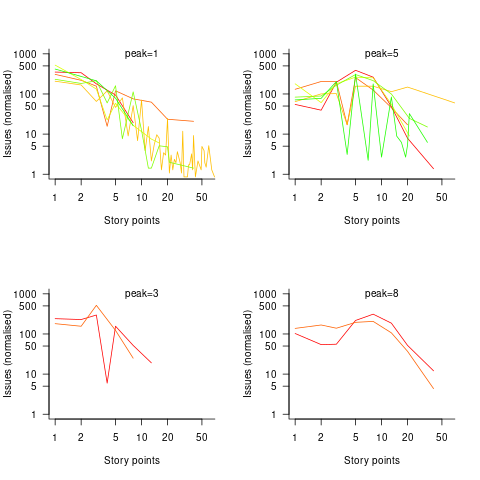
Are the projects with estimate peaks at 3 and 8 story points a quirk of this dataset, or is it to be expected that around 10% of projects will peak at one of these values?
For me, what jumps out of these plots is the number and extent of 4 story point estimates. Perhaps it’s just a visual effect, the actual number is an order of magnitude less than for 3 and 5 story points.
The plot below shows the percentage of estimated story points that are not Fibonacci numbers, sorted by project (the one project not showing has 0%; code+data):
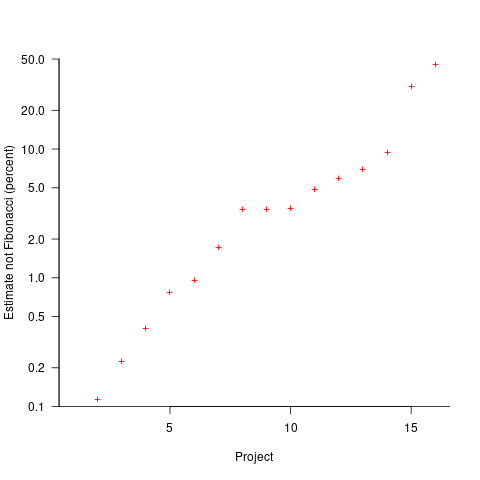
If nothing else, these plots provide a base to start from, and potentially claim to have seen this pattern before.
Rounding in reported task implementation time
There is lots of evidence that people often pick a round number when estimating the time needed to implement a task. Parkinson’s law suggests that reported actual implementation time will often also be a round number, e.g., report 30 minutes for a task that actually took 28 minutes.
If a task is estimated to take 1-hour, what is the distribution of reported implementations times? The analysis in this article uses the SiP task dataset, and similar patterns occur in other datasets.
The plot below shows the number of tasks having a given reported implementation time, for tasks estimated to take 1-hour, with main peaks labelled in red (reported times rounded to one decimal place and quarter hours; code+data):
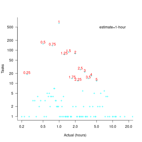
With 1-hour estimates, there is limited scope for a wide range of actual times (at least for times less than estimates). The labelled peaks contain 89% of 1-hour estimate tasks (1,525 tasks, 21% less than estimate, 44% equal estimate, 24% greater than estimate).
Tasks with larger estimated times are likely to take longer, creating more possible rounding peaks in the implementation time distribution. The plot below shows the number of tasks having a given reported implementation time, for tasks estimated to take 7-hour (i.e., 1-day), with main peaks labelled in red (reported times rounded to one decimal place and quarter hours; code+data):
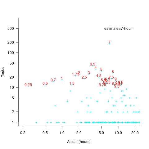
As expected, there are more peaks and implementation times are distributed over a larger range of values.
These plots suggest that many actual times are being rounded to 15-minute intervals. The plot below is based on the minute portion of the reported time (i.e., the hour part is ignored), and shows the fraction of tasks, for estimates of 1, 2, 3, 5, 7, and 14 hours, whose minute component of reported time has a given value (code+data):

For estimates of a few hours, around 90% of reported task time is on a 15-minute mark, while for 7- and 14-hour tasks the percentage drops to 80%.
If staff are manually entering task finish times, then some degree of rounding is to be expected. When the finish time is indirectly calculated, based on the submission of a completed form, there will be some fuzziness to the rounding number process.
Small team estimating in story points; a project dataset
Just before the end of last year a regular reader, Mr A., emailed to ask if I would be interested in analysing the software project data for the company he worked for. The wishing to be anonymous company sold physical products, and bespoke software that supported the business was written by a team of three.
Two factors made this dataset interesting, 1) it was for a small team, 2) story points were used for estimating tasks and actual time was recorded (I had not seen such data before).
There are probably hundreds of thousands of small software teams working in companies whose main line of business is far removed from software (a significant percentage of developers work within a small team supporting the activities of non-software companies; I cannot find the bls page listing developer employment across industry codes). These small teams are rarely studied. Software engineering research usually focuses on the practices of software based companies, or large software development projects, i.e., groups likely to be easily visible to external researchers.
To be widely applicable, evidence-based software engineering has to be of practical use to small development teams, not just large development groups.
The wide variety of opinions on the accuracy of story point estimates are unsupported by data; at least I have not yet been able to find any. Here was an opportunity to analyse story point estimates against actual hours.
The reason for analysing task implementation data is to help those involved understand what is going on, with the intent of improving processes. A small team presents two major challenges:
- relatively high levels of variability in the data. When there are only a few people working on a project, the impact of individual events can have a dramatic impact on project metrics, e.g., somebody going on holiday results in a big drop in work performed. Statistical analysis looks for general patterns in data, and small sample sizes have a higher variance than large sample sizes. With a large team, the impact of individual events tends to be smoothed out by the activities of many other events,
- the project lead of a small team is likely to have a good understanding of what is going on. Mr A. was always able to give me detailed explanations behind the patterns I found in the data. There is a lot more going on in a large team, and the team lead is unlikely to have a detailed understanding of everything.
The dataset contained some of the usual patterns found in other datasets (code+data):
- Round numbers. Actual task time finishing on 15/10/30/20 minute boundaries. With stories estimated at between one and five story points, there was little scope for round number use here.
- Consistent under/over estimation. A small sample size limited the chances of seeing both under and over estimation, and only under estimation was seen.
- Estimation accuracy. The factor of two/four accuracy pattern seen is close to that seen in data from other companies.
What did I learn from the analysis of this dataset?
I was pleased to see that the multiplication factors around estimation accuracy were similar to those seen with time-based estimates. I had no feel for how estimation accuracy might compare. We will have to wait and see whether the same pattern is found in other projects using story point estimates.
The analysis conversation for other project datasets had involved exchange of emails. Updating a Markdown formatted project analysis file has proved to be a more usable approach for the conversation between me and the domain expert. I used Visual Studio Code to edit this file and generate a pdf.
I asked Mr A. what would he thought was the most useful part of the analysis, for him.
Mr A. “The most useful part of the analysis? I think it was great to get an outsider’s perspective on the data.”
I hope that this dataset is the first of many from small team projects. With enough experience, it ought to be possible to create a template spreadsheet/markdown file that is generally usable for non-experts.
Evaluating Story point estimation error
If a task implementation estimate is expressed in time, various formula are available for evaluating how well the estimated time corresponds to the actual time.
When an estimate is expressed in story points, how might the estimate be evaluated when actual time is measured in hours?
The common practice of selecting story point values from a small set of integers (I have seen fractional values used) introduces quantization error into most estimates (around 30% of time estimates equal actual time), assuming that actual times are not constrained to a similar number of possible time values.
If we assume a linear mapping from estimated story points to actual time and an ideal estimator (let’s assume that 1 story point is equivalent to 1 hour), then a lower bound on the error can be calculated.
Our ideal estimator is able to exactly predict the actual time. However, the use of story points means that this exact prediction has to be rounded to one of a small set of integer values. Let’s assume that our ideal estimator rounds to the story point value that is closest to the exact prediction, e.g., all story points predicted to take up to 1.5 are estimated at 1 story point.
What is the mean error of the estimates made by this ideal, rounded, estimator?
The available evidence shows that the distribution of tasks having a given actual implementation time roughly has the form of a geometric (the discrete form of exponential) or negative binomial distribution. The plot below shows a geometric and negative binomial distribution, with distinct colors over the range where values are rounded to the same closest integer (dots are at 1-minute intervals, code):
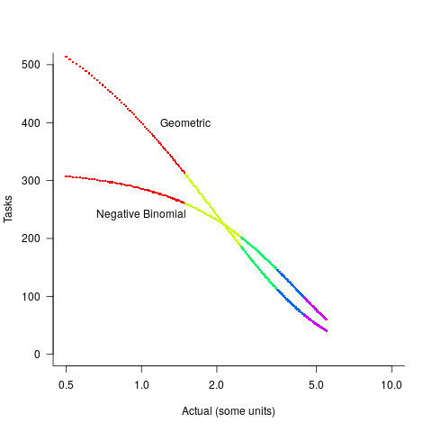
Having picked a distribution for actual times, we can calculate the number of tasks estimated to require, for instance, 1 story point, but actually taking 1 hour, 1 hr 1 min, 1 hr 2 min, …, 1 hr 30 min. The mean error can be calculated over each pair of estimate/actual, for one to five story points (in this example). The table below lists the mean error for two actual distributions, calculated using four common metrics: squared error (SE), absolute error (AE), absolute percentage error (APE), and relative error (RE); code:
Distribution SE AE APE RE Geometric 0.087 0.26 0.17 0.20 Negative Binomial 0.086 0.25 0.14 0.16 |
A few minutes difference in a 1 SP estimate is a larger error than the same number of minutes in a two or more SP estimate, combined with most tasks take a small amount of time, means that error estimation is dominated by inaccuracies in estimating small tasks.
In practice, the range of actual times, for a given estimate, is better approximated by a percentage of the estimated time (50% is used below), and the number of tasks having a given actual value for a given estimate, approximated by a triangular distribution (a cubic equation was used for the following calculation). The plot below shows the distribution of estimation points around a given number of story points (at 1-minute intervals), and the geometric and negative binomial distribution (compare against plot above to work out which is which; code):
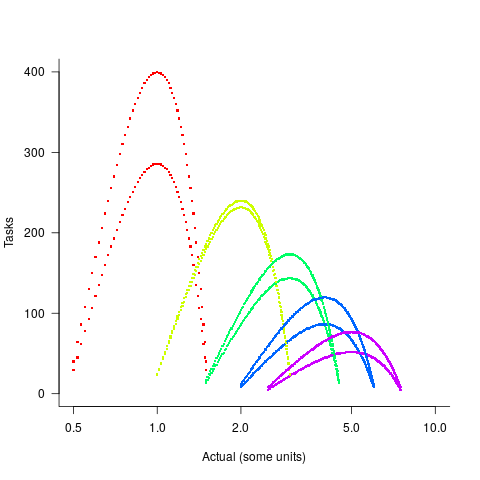
The following table lists of mean errors:
Distribution SE AE APE RE Geometric 0.52 0.55 0.13 0.13 Negative Binomial 0.62 0.61 0.13 0.14 |
When the error in the actual is a percentage of the estimate, larger estimates have a much larger impact on absolute accuracy; see the much larger SE and AE values. The impact on the relative accuracy metrics appears to be small.
Is evaluating estimation error useful, when estimates are given in story points?
While it’s possible to argue for and against, the answer is that usefulness is in the eye of the beholder. If development teams find the information useful, then it is useful; otherwise not.
Shopper estimates of the total value of items in their basket
Agile development processes break down the work that needs to be done into a collection of tasks (which may be called stories or some other name). A task, whose implementation time may be measured in hours or a few days, is itself composed of a collection of subtasks (which may in turn be composed of subsubtasks, and so on down).
When asked to estimate the time needed to implement a task, a developer may settle on a value by adding up estimates of the effort needed to implement the subtasks thought to be involved. If this process is performed in the mind of the developer (i.e., not by writing down a list of subtask estimates), the accuracy of the result may be affected by the characteristics of cognitive arithmetic.
Humans have two cognitive systems for processing quantities, the approximate number system (which has been found to be present in the brain of many creatures), and language. Researchers studying the approximate number system often ask subjects to estimate the number of dots in an image; I recently discovered studies of number processing that used language.
In a study by Benjamin Scheibehenne, 966 shoppers at the checkout counter in a grocery shop were asked to estimate the total value of the items in their shopping basket; a subset of 421 subjects were also asked to estimate the number of items in their basket (this subset were also asked if they used a shopping list). The actual price and number of items was obtained after checkout.
There are broad similarities between shopping basket estimation and estimating task implementation time, e.g., approximate idea of number of items and their cost. Does an analysis of the shopping data suggest ideas for patterns that might be present in software task estimate data?
The left plot below shows shopper estimated total item value against actual, with fitted regression line (red) and estimate==actual (grey); the right plot shows shopper estimated number of items in their basket against actual, with fitted regression line (red) and estimate==actual (grey) (code+data):
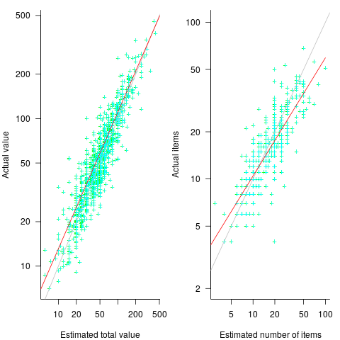
The model fitted to estimated total item value is:  , which differs from software task estimates/actuals in always underestimating over the range measured; the exponent value,
  , is at the upper range of those seen for software task estimates.
The model fitted to estimated number of items in the basket is:  . This pattern, of underestimating small values and overestimating large values is seen in software task estimation, but the exponent of
  is much smaller.
Including the estimated number of items in the shopping basket,  , in a model for total value produces a slightly better fitting model:
  , which explains 83% of the variance in the data (use of a shopping list had a relatively small impact).
The accuracy of a software task implementation estimate based on estimating its subtasks dependent on identifying all the subtasks, or having a good enough idea of the number of subtasks. The shopping basket study found a pattern of inaccuracies in estimates of the number of recently collected items, which has been seen before. However, adding to the Shopping model only reduced the unexplained variance by a few percent.
Would the impact of adding an estimate of the number of subtasks to models of software task estimates also only be a few percent? A question to add to the already long list of unknowns.
Like task estimates, round numbers were often given as estimate values; see code+data.
The same study also included a laboratory experiment, where subjects saw a sequence of 24 numbers, presented one at a time for 0.5 seconds each. At the end of the sequence, subjects were asked to type in their best estimate of the sum of the numbers seen (other studies asked subjects to type in the mean). Each subject saw 75 sequences, with feedback on the mean accuracy of their responses given after every 10 sequences. The numbers were described as the prices of items in a shopping basket. The values were drawn from a distribution that was either uniform, positively skewed, negatively skewed, unimodal, or bimodal. The sequential order of values was either increasing, decreasing, U-shaped, or inversely U-shaped.
Fitting a regression model to the lab data finds that the distribution used had very little impact on performance, and the sequence order had a small impact; see code+data.
Over/under estimation factor for ‘most estimates’
When asked to estimate the time taken to perform a software development related task, people regularly over or under estimate. What range of over/under estimation falls within the bounds of the term ‘most estimates’, i.e., the upper/lower bounds of the ratio  (an overestimate occurs when
  , an underestimate when
  )?
)?
On Twitter, I have been citing a factor of two for over/under time estimates. This factor of two involves some assumptions and a personal interpretation.
The following analysis is based on the two major software task effort estimation datasets: SiP and CESAW. The tasks in both datasets are for internal projects (i.e., no tendering against competitors), and require at most a few hours work.
The following analysis is based on the SiP data.
Of the 8,252 unique tasks in the SiP data, 30% are underestimates, 37% exact, and 33% overestimates.
How do we go about calculating bounds for the over/under factor of most estimates (a previous post discussed calculating an accuracy metric over all estimates)?
A simplistic approach is to average over each of the overestimated and underestimated tasks. The plot below shows hours estimated against the ratio actual/estimated, for each task (code+data):
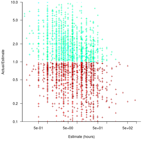
Averaging the over/under estimated tasks separately (using the geometric mean) gives 0.47 and 1.9 respectively, i.e., tasks are over/under estimated by a factor of two.
This approach fails to take into account the number of estimates that are over/under/equal, i.e., it ignores likelihood information.
A regression model takes into account the distribution of values, and we could adopt the fitted model’s prediction interval as the over/under confidence intervals. The prediction interval is the interval within which other observations are expected to fall, with some probability (R’s predict function uses one standard deviation).
The plot below shows a fitted regression model and prediction intervals at one standard deviation (68.3%) and two standard deviations (95%); the faint grey line shows Estimate == Actual (code+data):
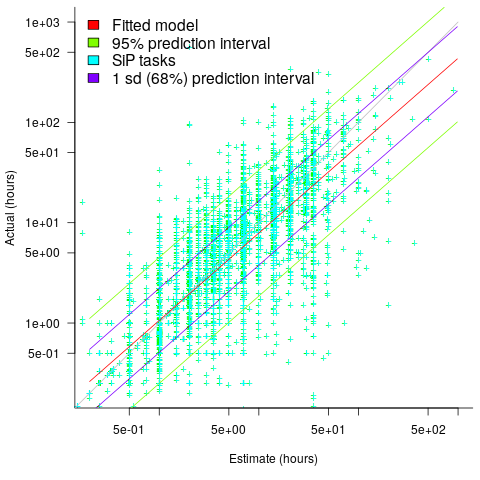
The fitted model tilts down from the upward direction of the Estimate == Actual line, consequently the over/under estimation factor depends on the size of the estimate. The table below lists the over/under estimation factor for low/high estimates at one & two standard deviations (68.3 and 95% probability).
People like simple answers (i.e., single values) and the mean value is a commonly used technique of summarising many values. The task estimate values are unevenly distributed and weighting the mean by the distribution of estimated values is more representative than, say, an evenly distributed set of estimates. The 5th and 6th columns in the table below list the weighted means at one/two standard deviations (the CESAW columns are the values for all projects in the CESAW data).
          1 sd           2 sd        Weighted mean       CESAW
       Low    High   Low    High     1 sd    2 sd     1 sd   2 sd
Over   0.56   0.24   0.27   0.11     0.46    0.25     0.29   0.1
Under 2.4 1.0 4.9 2.0 2.00 4.1 2.4 6.5 |
The weighted means for over/under estimates are close to a factor of two of the actual (divide/multiply) within one standard deviation (68.3%), and a factor of four within two standard deviations (95%).
Why choose to give the one standard deviation factor, rather than the two? People talk of “most estimates”, but what percentage range does ‘most’ map to? I have tended to think of ‘most’ as more than two-thirds, e.g., at least one standard deviation (a recent study suggests that ‘most’ usage peaks at 80-85%), and I think of two standard deviations as ‘nearly all’ (i.e., 95%; there are probably people who call this ‘most’).
Perhaps a between two and four is a more appropriate answer (particularly since the bounds are wider for the CESAW data). Suggestions welcome.
Evaluating estimation performance
What is the best way to evaluate the accuracy of an estimation technique, given that the actual values are known?
Estimates are often given as point values, and accuracy scoring functions (for a sequence of estimates) have the form }") , where
, where  is the number of estimated values,
  the estimates, and
  the actual values; smaller
  is better.
Commonly used scoring functions include:
=(E-A)^2") , known as squared error (SE)
, known as squared error (SE)=delim{|}{E-A}{|}") , known as absolute error (AE)
, known as absolute error (AE)=delim{|}{E-A}{|}/A") , known as absolute percentage error (APE)
, known as absolute percentage error (APE)=delim{|}{E-A}{|}/E") , known as relative error (RE)
, known as relative error (RE)
APE and RE are special cases of: =delim{|}{1-(A/E)^{beta}}{|}") , with
, with  and
and  respectively.
Let’s compare three techniques for estimating the time needed to implement some tasks, using these four functions.
Assume that the mean time taken to implement previous project tasks is known,  . When asked to implement a new task, an optimist might estimate 20% lower than the mean,
  , while a pessimist might estimate 20% higher than the mean,
  . Data shows that the distribution of the number of tasks taking a given amount of time to implement is skewed, looking something like one of the lines in the plot below (code):
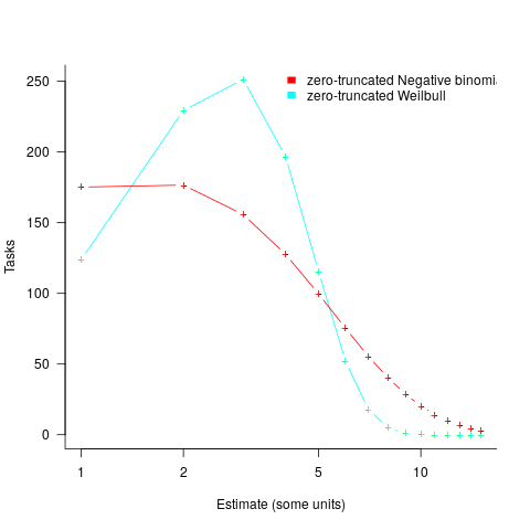
We can simulate task implementation time by randomly drawing values from a distribution having this shape, e.g., zero-truncated Negative binomial or zero-truncated Weibull. The values of  and
and  are calculated from the mean, , of the distribution used (see code for details). Below is each estimator’s score for each of the scoring functions (the best performing estimator for each scoring function in bold; 10,000 values were used to reduce small sample effects):
    SE   AE   APE   RE

  2.73 1.29 0.51 0.56

 2.31 1.23 0.39 0.68

  2.70 1.37 0.36 0.86
Surprisingly, the identity of the best performing estimator (i.e., optimist, mean, or pessimist) depends on the scoring function used. What is going on?
The analysis of scoring functions is very new. A 2010 paper by Gneiting showed that it does not make sense to select the scoring function after the estimates have been made (he uses the term forecasts). The scoring function needs to be known in advance, to allow an estimator to tune their responses to minimise the value that will be calculated to evaluate performance.
The mathematics involves Bregman functions (new to me), which provide a measure of distance between two points, where the points are interpreted as probability distributions.
Which, if any, of these scoring functions should be used to evaluate the accuracy of software estimates?
In software estimation, perhaps the two most commonly used scoring functions are APE and RE. If management selects one or the other as the scoring function to rate developer estimation performance, what estimation technique should employees use to deliver the best performance?
Assuming that information is available on the actual time taken to implement previous project tasks, then we can work out the distribution of actual times. Assuming this distribution does not change, we can calculate APE and RE for various estimation techniques; picking the technique that produces the lowest score.
Let’s assume that the distribution of actual times is zero-truncated Negative binomial in one project and zero-truncated Weibull in another (purely for convenience of analysis, reality is likely to be more complicated). Management has chosen either APE or RE as the scoring function, and it is now up to team members to decide the estimation technique they are going to use, with the aim of optimising their estimation performance evaluation.
A developer seeking to minimise the effort invested in estimating could specify the same value for every estimate. Knowing the scoring function (top row) and the distribution of actual implementation times (first column), the minimum effort developer would always give the estimate that is a multiple of the known mean actual times using the multiplier value listed:
                   APE   RE

Negative binomial  1.4   0.5

Weibull            1.2   0.6
For instance, management specifies APE, and previous task/actuals has a Weibull distribution, then always estimate the value  .
.
What mean multiplier should Esta Pert, an expert estimator aim for? Esta’s estimates can be modelled by the equation ") , i.e., the actual implementation time multiplied by a random value uniformly distributed between 0.5 and 2.0, i.e., Esta is an unbiased estimator. Esta’s table of multipliers is:
, i.e., the actual implementation time multiplied by a random value uniformly distributed between 0.5 and 2.0, i.e., Esta is an unbiased estimator. Esta’s table of multipliers is:
                   APE     RE

Negative binomial  1.0   0.7

Weibull                     1.0     0.7
A company wanting to win contracts by underbidding the competition could evaluate Esta’s performance using the RE scoring function (to motivate her to estimate low), or they could use APE and multiply her answers by some fraction.
In many cases, developers are biased estimators, i.e., individuals consistently either under or over estimate. How does an implicit bias (i.e., something a person does unconsciously) change the multiplier they should consciously aim for (having analysed their own performance to learn their personal percentage bias)?
The following table shows the impact of particular under and over estimate factors on multipliers:
                 0.8 underestimate bias   1.2 overestimate bias

Score function          APE   RE            APE   RE

Negative binomial        1.3   0.9           0.8   0.6

Weibull                 1.3       0.9           0.8   0.6
Let’s say that one-third of those on a team underestimate, one-third overestimate, and the rest show no bias. What scoring function should a company use to motivate the best overall team performance?
The following table shows that neither of the scoring functions motivate team members to aim for the actual value when the distribution is Negative binomial:
                    APE      RE

Negative binomial    1.1     0.7

Weibull                               1.0       0.7
One solution is to create a bespoke scoring function for this case. Both APE and RE are special cases of a more general scoring function (see top). Setting  in this general form creates a scoring function that produces a multiplication factor of 1 for the Negative binomial case.
How large an impact does social conformity have on estimates?
People experience social pressure to conform to group norms. How big an impact might social pressure have on a developer’s estimate of the effort needed to implement some functionality?
If a manager suggests that the effort likely to be required is large/small, I would expect a developer to respond accordingly (even if the manager is thought to be incompetent; people like to keep their boss happy). Of course, customer opinions are also likely to have an impact, but what about fellow team members, or even the receptionist. Until somebody runs the experiments, we are going to have to do with non-software related tasks.
A study by Molleman, Kurversa, and van den Bos asked subjects (102 workers on Mechanical Turk) to estimate the number of animals in an image (which contained between 50 and 100 ants, flamingos, bees, cranes or crickets). Subjects were given 30 seconds to respond, and after typing their answer they were told that “another participant had estimated X“, and given 45 seconds to give a second estimate. The ‘social pressure’ estimate, X, was chosen to be around 15-25% larger/smaller than the estimate given (values from a previous experiment were randomly selected).
The plot below shows the number of second estimates where there was a given percentage change between the first and second estimates, red line is a loess fit; the formula used is  (code+data):
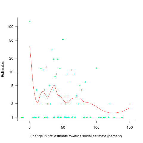
Around 25% of second estimates were unchanged, and 2% were changed to equal the social estimate. In two cases the second estimate was less than the first, and in eleven cases it was larger than the social estimate. Both the mean and median for shift towards the social estimate were just over 30% of the difference between the first estimate and the social estimate.
As with previous estimating studies, a few round numbers were often chosen. I was interested in finding out what impact the use of a round number value for the first estimate, or the social estimate, might have on the change in estimated value. The best regression model I could find showed that if the first estimate was exactly divisible by 5 (or 10), then the second estimate was likely to be around 5% larger. In fact divisible-by-5 was the only variable that had any predictive power.
My initial hypothesis was that the act of choosing a round number is an expression of uncertainty, and that this uncertainty increases the impact of the social estimate (when making the second estimate). An analysis of later experiments suggested that this pattern was illusionary (see below).
Modelling estimate values, rather than their differences, the equation:  explains nearly all the variance present in the data.
Two weeks after the first experiment, all 102 subjects were asked to repeat the experiment (they each saw the same images, in the same order, and social estimates as in the first study); 69 subjects participated. Nine months after the first experiment, subjects were asked to repeat the experiment again; 47 subjects participated, again with each subject seeing the same images in the same order, and social estimates. Thirty-five subjects participated in all three experiments.
To what extent were subjects consistently influenced by the social estimate, across three identical sessions? The Pearson correlation coefficient between both the first/second experiment, and the first/third experiment, was around 0.6.
The impact of round numbers was completely different, i.e., no impact on the second, and a -7% impact on the third (i.e., a reduced change). So much for my initial hypothesis.
The exponents in the above equation did not change much for the data from the second and third reruns of the experiment.
The variability in the social estimates used in these experiments, involving image contents, differs from software estimates in that they were only 12-25% different from the first estimate. Software estimates often differ by significantly larger amounts (in fact, a 12% difference would probably be taken as agreement).
With some teams, people meet to thrash out a team estimate. Data is sometimes available on the final estimate, but data on the starting values is very hard to come by. Pointers to experiments where social estimates are significantly different (i.e., greater than 50%) from the ones given by subjects welcome.
Recent Comments