Archive
Detailed management data on 1,211 software projects
Until April this year there were only two non-trivial publicly available software project datasets (i.e., Sip and CESAW) containing software project data relating to human effort, e.g., people time, elapsed time, and tasks performed. The SiP data contains 10-years of software development tasks by one company, and the CESAW data contains the tasks involved in implementing 45 software projects.
Two months ago the Software Excellence Alliance released the SEA Data Warehouse (the CESAW data is roughly a 10% subset of SEA). This post compares software project size from the perspective of various management related features.
An analysis of pre-LLM project development is still relevant because many project behavior patterns are driven by interactions with the outside world. Also, time spent writing code is often small part of project development.
The headline summary is that there is development-phase/estimates/actuals/start-time/end-time/person/team/etc information for the 679,904 tasks involved in implementing 1,211 software projects.
The projects were developed using the Team Software Process (TSP). This is an iterative development process that uses development phases similar to the Waterfall process, with weekly meeting that monitor progress using earned-value management. Given that the work-breakdown structure (WBS) is used to break down a project into a hierarchy of smaller and smaller components, these projects are US Department of Defense related.
The plot below shows, for each of the 1,211 projects (sorted by number of plans, in black), the number of tasks (blue), WBS (green), and deleted plans (red) ( ; code+data):
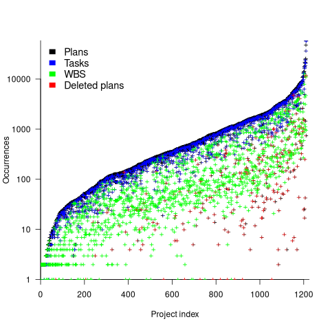
The average ratio of  is 8.4 (standard deviation 23). An exponential or power law (not Weibull) can be fitted to portions of the distribution of project sizes, measured in number of plans or tasks. If project size really does follow a single common distribution, a much larger sample size will be needed to reliably fit it.
The plot below shows, for each project (sorted by total person hours, in red), the number of elapsed days from start of first to end of last task (green), and number of people who worked on at least one task (blue) (projects implemented by a single person do not have consistent time data; code+data):
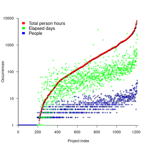
For a given number of person hours worked on a project, there is an order of magnitude variation in elapsed days and number of people who worked on at least one task.
This dataset contains a huge amount of detail, and I’m sure there are lots of patterns to be found. But, what are the important questions to ask, that would be useful to project managers. When I ask managers what project questions they would like answers, the response is often one of quizzical uncertainty. There are plenty of people promoting their opinions, and it’s very rare to encounter anybody asking meaningful questions.
Projects are worked on in fits and starts
Companies whose business is designing, developing, and maintaining custom software applications (i.e., a software house) have the difficult job of keeping their expensive employees busy with paying work. Work on an existing project may be held up for various reasons, and the start date of new projects is invariably uncertain.
A solution to the on/off nature of project work is for staff to distribute their time across multiple projects. If one project is held up, there is another project available for them to book their time to.
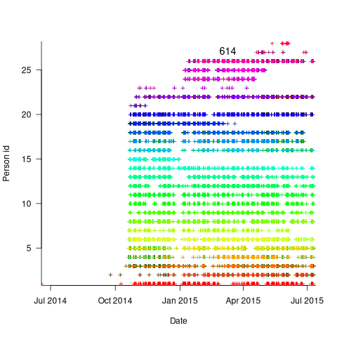
The plot below is for project 614 in the CESAW dataset, and shows the days on which 28 people worked on this project between July 2014 and July (code+data):
The published models of the software development lifecycle are based on perceptions of the workings of large DOD and NASA projects from the 1960s and 1970s. These projects are treated as self-contained entities, with people being available when needed and individually interchangeable. This perception fits with the software physics thinking of the time, along with the early 1960s work of Norden, and the use of differential equations to model the evolution of project manpower. These models fitted the small amount of available data as well as several other models. With some hand waving it is possible to make models such as the Putnam model look good.
With 28 people working on project 614, it’s possible that individual contributions don’t have a big impact on totals, i.e., the total time spent per week (say) does not fluctuate widely. The plot below shows the total hours per week spent on design, coding and test (total project time as roughly three staff years; code+data):
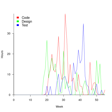
Plenty of wide fluctuations, plus some expected large drops in time spent on the project. For instance, a big drop in all activities around Christmas, and a smaller dip around Thanksgiving.
Having 28 people work on a three-person year project does seem a bit extreme (average of seven-weeks per person). On the other hand, I may be out of date, not having been a team member on a large project in decades.
The total effort required by the projects in the CESAW dataset range from three-person months to three-person years, which I suspect (no data on this question) straddles the range of time spent on the majority of software projects. The projects mostly involve people spending a non-large percentage of time on a project. The data is anonymised on a project basis, and it is not possible to count the number of projects a person is working on at any time.
To summarise: Building a good enough model of software project staffing requires taking into account organization wide staffing priorities. Existing models don’t do this.
Over/under estimation factor for ‘most estimates’
When asked to estimate the time taken to perform a software development related task, people regularly over or under estimate. What range of over/under estimation falls within the bounds of the term ‘most estimates’, i.e., the upper/lower bounds of the ratio  (an overestimate occurs when
  , an underestimate when
  )?
)?
On Twitter, I have been citing a factor of two for over/under time estimates. This factor of two involves some assumptions and a personal interpretation.
The following analysis is based on the two major software task effort estimation datasets: SiP and CESAW. The tasks in both datasets are for internal projects (i.e., no tendering against competitors), and require at most a few hours work.
The following analysis is based on the SiP data.
Of the 8,252 unique tasks in the SiP data, 30% are underestimates, 37% exact, and 33% overestimates.
How do we go about calculating bounds for the over/under factor of most estimates (a previous post discussed calculating an accuracy metric over all estimates)?
A simplistic approach is to average over each of the overestimated and underestimated tasks. The plot below shows hours estimated against the ratio actual/estimated, for each task (code+data):
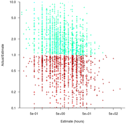
Averaging the over/under estimated tasks separately (using the geometric mean) gives 0.47 and 1.9 respectively, i.e., tasks are over/under estimated by a factor of two.
This approach fails to take into account the number of estimates that are over/under/equal, i.e., it ignores likelihood information.
A regression model takes into account the distribution of values, and we could adopt the fitted model’s prediction interval as the over/under confidence intervals. The prediction interval is the interval within which other observations are expected to fall, with some probability (R’s predict function uses one standard deviation).
The plot below shows a fitted regression model and prediction intervals at one standard deviation (68.3%) and two standard deviations (95%); the faint grey line shows Estimate == Actual (code+data):
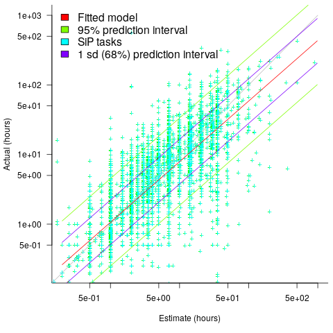
The fitted model tilts down from the upward direction of the Estimate == Actual line, consequently the over/under estimation factor depends on the size of the estimate. The table below lists the over/under estimation factor for low/high estimates at one & two standard deviations (68.3 and 95% probability).
People like simple answers (i.e., single values) and the mean value is a commonly used technique of summarising many values. The task estimate values are unevenly distributed and weighting the mean by the distribution of estimated values is more representative than, say, an evenly distributed set of estimates. The 5th and 6th columns in the table below list the weighted means at one/two standard deviations (the CESAW columns are the values for all projects in the CESAW data).
          1 sd           2 sd        Weighted mean       CESAW
       Low    High   Low    High     1 sd    2 sd     1 sd   2 sd
Over   0.56   0.24   0.27   0.11     0.46    0.25     0.29   0.1
Under 2.4 1.0 4.9 2.0 2.00 4.1 2.4 6.5 |
The weighted means for over/under estimates are close to a factor of two of the actual (divide/multiply) within one standard deviation (68.3%), and a factor of four within two standard deviations (95%).
Why choose to give the one standard deviation factor, rather than the two? People talk of “most estimates”, but what percentage range does ‘most’ map to? I have tended to think of ‘most’ as more than two-thirds, e.g., at least one standard deviation (a recent study suggests that ‘most’ usage peaks at 80-85%), and I think of two standard deviations as ‘nearly all’ (i.e., 95%; there are probably people who call this ‘most’).
Perhaps a between two and four is a more appropriate answer (particularly since the bounds are wider for the CESAW data). Suggestions welcome.
The CESAW dataset: a brief introduction
I have found that the secret for discovering data treasure troves is persistently following any leads that appear. For instance, if a researcher publishes a data driven paper, then check all their other papers. The paper: Composing Effective Software Security Assurance Workflows contains a lot of graphs and tables, but no links to data, however, one of the authors (William R. Nichols) published The Cost and Benefits of Static Analysis During Development which links to an amazing treasure trove of project data.
My first encounter with this data was this time last year, as I was focusing on completing my Evidence-based software engineering book. Apart from a few brief exchanges with Bill Nichols the technical lead member of the team who obtained and originally analysed the data, I did not have time for any detailed analysis. Bill was also busy, and we agreed to wait until the end of the year. Bill’s and my paper: The CESAW dataset: a conversation is now out, and focuses on an analysis of the 61,817 task and 203,621 time facts recorded for the 45 projects in the CESAW dataset.
Our paper is really an introduction to the CESAW dataset; I’m sure there is a lot more to be discovered. Some of the interesting characteristics of the CESAW dataset include:
- it is the largest publicly available project dataset currently available, with six times as many tasks as the next largest, the SiP dataset. The CESAW dataset involves the kind of data that is usually encountered, i.e., one off project data. The SiP dataset involves the long term evolution of one company’s 20 projects over 10-years,
- it includes a lot of information I have not seen elsewhere, such as: task interruption time and task stop/start {date/time}s (e.g., waiting on some dependency to become available)
- four of the largest projects involve safety critical software, for a total of 28,899 tasks (this probably more than two orders of magnitude more than what currently exists). Given all the claims made about the development about safety critical software being different from other kinds of development, here is a resource for checking some of the claims,
- the tasks to be done, to implement a project, are organized using a work-breakdown structure. WBS is not software specific, and the US Department of Defense require it to be used across all projects; see MIL-STD-881. I will probably annoy those in software management by suggesting the one line definition of WBS as: Agile+structure (WBS supports iteration). This was my first time analyzing WBS project data, and never having used it myself, I was not really sure how to approach the analysis. Hopefully somebody familiar with WBS will extract useful patterns from the data,
- while software inspections are frequently talked about, public data involving them is rarely available. The WBS process has inspections coming out of its ears, and for some projects inspections of one kind or another represent the majority of tasks,
- data on the kinds of tasks that are rarely seen in public data, e.g., testing, documentation, and design,
- the 1,324 defect-facts include information on: the phase where the mistake was made, the phase where it was discovered, and the time taken to fix.
As you can see, there is lots of interesting project data, and I look forward to reading about what people do with it.
Once you have downloaded the data, there are two other sources of information about its structure and contents: the code+data used to produce the plots in the paper (plus my fishing expedition code), and a CESAW channel on the Evidence-based software engineering Slack channel (no guarantees about response time).
Recent Comments