Archive
Modeling visual studio C++ compile times
Last week I spotted an interesting article on the compile-time performance of C++ compilers running under Microsoft Windows. The author had obviously put a lot of work into gathering the data, and had taken care to have multiple runs to reduce the impact of random effects (128 runs to be exact); but, as if often the case, the analysis of the data was lackluster. I posted a comment asking for the data, and a link was posted the next day 🙂
The compilers benchmarked were: Visual Studio 2015, Visual Studio 2017 and clang 7.0.1; the compilers were configured to target: C++20, C++17, C++14, C++11, C++03, or C++98. The source code used was 100 system headers.
If we are interested in understanding the contribution of each component to overall compile-time, the obvious fist regression model to build is:

where:  are the different headers,
  the different compilers and
  the different target languages. There might be some interaction between variables, so something more complicated was tried first; the final fitted model was (code+data):

where  is a constant (the
 Intercept in R’s summary output). The following is a list of normalised numbers to plug into the equation (clang is the default compiler and C++03 the default language, and so do not appear in the list, the : symbol represents the multiplication; only a few of the 100 headers are listed, details are available):
Estimate Std. Error t value Pr(>|t|) (Intercept) headerany 1.000000000 0.051100398 headerarray headerassert.h 0.522336397 -0.654056185 ... headerwctype.h headerwindows.h -0.648095154 1.304270250 compilerVS15 compilerVS17 -0.185795534 -0.114590143 languagec++11 languagec++14 0.032930014 0.156363433 languagec++17 languagec++20 0.192301727 0.184274629 languagec++98 compilerVS15:languagec++11 0.001149643 -0.058735591 compilerVS17:languagec++11 compilerVS15:languagec++14 -0.038582437 -0.183708714 compilerVS17:languagec++14 compilerVS15:languagec++17 -0.164031495 NA compilerVS17:languagec++17 compilerVS15:languagec++20 -0.181591418 NA compilerVS17:languagec++20 compilerVS15:languagec++98 -0.193587045 0.062414667 compilerVS17:languagec++98 0.014558295 |
As an example, the (normalised) time to compile wchar.h using VS15 with languagec++11 is:
1-0.514807638-0.183862162+0.033951731-0.059720131
Each component adds/substracts to/from the normalised mean.
Building this model didn’t take long. While waiting for the kettle to boil, I suddenly realised that an additive model was probably inappropriate for this problem; oops. Surely the contribution of each component was multiplicative, i.e., components have a percentage impact to performance.
A quick change to the form of the fitted model:
 = k+header_x+compiler_y+language_z+compiler_y*language_z")
Taking the exponential of both side, the fitted equation becomes:

The numbers, after taking the exponent, are:
(Intercept) headerany 9.724619e+08 1.051756e+00 ... headerwctype.h headerwindows.h 3.138361e-01 2.288970e+00 compilerVS15 compilerVS17 7.286951e-01 7.772886e-01 languagec++11 languagec++14 1.011743e+00 1.049049e+00 languagec++17 languagec++20 1.067557e+00 1.056677e+00 languagec++98 compilerVS15:languagec++11 1.003249e+00 9.735327e-01 compilerVS17:languagec++11 compilerVS15:languagec++14 9.880285e-01 9.351416e-01 compilerVS17:languagec++14 compilerVS15:languagec++17 9.501834e-01 NA compilerVS17:languagec++17 compilerVS15:languagec++20 9.480678e-01 NA compilerVS17:languagec++20 compilerVS15:languagec++98 9.402461e-01 1.058305e+00 compilerVS17:languagec++98 1.001267e+00 |
Taking the same example as above: wchar.h using VS15 with c++11. The compile-time (in cpu clock cycles) is:
9.724619e+08*3.138361e-01*7.286951e-01*1.011743e+00*9.735327e-01
Now each component causes a percentage change in the (mean) base value.
Both of these model explain over 90% of the variance in the data, but this is hardly surprising given they include so much detail.
In reality compile-time is driven by some combination of additive and multiplicative factors. Building a combined additive and multiplicative model is going to be like wrestling an octopus, and is left as an exercise for the reader 🙂
Given a choice between these two models, I think the multiplicative model is probably closest to reality.
Teaching basic data analysis to programmers: summer internship
Software engineering is one of the topics in this year’s summer internships being sponsored by R-Studio. The spec says: “Data Science Training for Software Engineers – Develop course materials to teach basic data analysis to programmers using software engineering problems and data sets.”
It’s good to see interest in data analysis of software engineering data start to gain traction.
What topics might basic data analysis for programmers include? I have written about statistical techniques that I think are useful in software engineering, but I don’t think this list would be regarded as basic. Techniques that are think are basic are:
- a picture is worth a thousand words, so obviously visualization is a major topic,
- building regression models is good for helping to understand what is going on.
Anything else? Well, I don’t know.
An alternative approach to teaching basic data analysis is to give examples of the kind of useful things it can be used to do. Software developers are fast learners, and given the motivation have the skills needed to find and learn techniques that they think are of use. In a basic course, I would put the emphasis on motivating developers to think that data analysis can help them do a better job.
I would NOT, repeat, not, include any material on machine learning. Software engineering data sets tend to be too small to obtain reliable results from machine learning, and I don’t want to encourage clueless button pushers.
What are the desirable skills in the summer intern? I would say that being able to write readable material is the most important, with statistical knowledge ranked second; the level of software engineering knowledge is unimportant. Data analysis tends to follow the same pattern whatever the subject; so it’s important to get somebody who knows about data analysis.
A social science major is the obvious demographic for this intern (they do lots of data analysis); the last people to consider are students majoring in a computing subject.
Choosing between two reasonably fitting probability distributions
I sometimes go fishing for a probability distribution to fit some software engineering data I have. Why would I want to spend time fishing for a probability distribution?
Data comes from events that are driven by one or more processes. Researchers have studied the underlying patterns present in many processes and in some cases have been able to calculate which probability distribution matches the pattern of data that it generates. This approach starts with the characteristics of the processes and derives a probability distribution. Often I don’t really know anything about the characteristics of the processes that generated the data I am looking at (but I can often make what I like to think are intelligent guesses). If I can match the data with a probability distribution, I can use what is known about processes that generate this distribution to get some ideas about the kinds of processes that could have generated my data.
Around nine-months ago, I learned about the Conway–Maxwell–Poisson distribution (or COM-Poisson). This looked as-if it might find some use in fitting software engineering data, and I added it to my list of distributions to keep in mind. I saw that the R package COMPoissonReg supports the fitting of COM-Poisson distributions.
This week I came across one of the papers, about COM-Poisson, that I was reading nine-months ago, and decided to give it a go with some count-data I had.
The Poisson distribution involves count-data, i.e., non-negative integers. Lots of count-data samples are well described by a Poisson distribution, and it is one of the basic distributions supported by statistical packages. Processes described by a Poisson distribution are memory-less, in that the probability of an event occurring are independent of when previous events occurred. When there is a connection between events, the Poisson distribution is not such a good fit (depending on the strength of the connection between events).
While a process that generates count-data may not meet the requirements needed to be exactly described by a Poisson distribution, the behavior may be close enough to give good-enough results. R supports a quasipoisson distribution to help handle the ‘near-misses’.
Sometimes count-data has a distribution that looks nothing like a Poisson. The Negative-binomial distribution is the obvious next choice to try (this can be viewed as a combination of different Poisson distributions; another combination is the Poisson inverse gaussian distribution).
The plot below (from a paper analyzing usage of record data structures in Racket; Tobias Pape kindly sent me the data) shows the number of Racket structure types that contain a given number of fields (red pluses), along with lines showing fitted Negative binomial and COM-Poisson distributions (code+data):
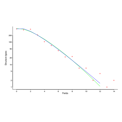
I’m interested in understanding the processes that are generating the data, and having two distributions do such a reasonable job of fitting the data has given me more possible distinct explanations for what is going on than I wanted (if I were interested in prediction, then either distribution looks like it would do a good-enough job).
What are the characteristics of the processes that generate data having each of the distributions?
- A Negative binomial can be viewed as a combination of Poisson distributions (the combination having a Gamma distribution). We could create a story around multiple processes being responsible for the pattern seen, with each of these processes having the impact of a Poisson distribution. Sounds plausible.
- A COM-Poisson distribution can be viewed as a Poisson distribution which is length dependent. We could create a story around the probability of a field being added to a structure type being dependent on the number of existing fields it contains. Sounds plausible (it’s a slightly different idea from preferential attachment).
When fitting a distribution to data, I usually go with the ‘brand-name’ distributions (i.e., the one with most name recognition, provided it matches well enough; brand names are an easier sell then the less well known names).
The Negative binomial distribution is the brand-name here. I had not heard of the COM-Poisson distribution until nine-months ago.
Perhaps the authors of the Racket analysis paper will come up with a theory that prefers one of these distributions, or even suggests another one.
Readers of my evidence-based software engineering book need to be aware of my brand-name preference in some of the data fitting that occurs.
Wanted: 99 effort estimation datasets
Every now and again, I stumble upon a really interesting dataset. Previously, when this happened I wrote an extensive blog post; but the SiP dataset was just too big and too detailed, it called out for a more expansive treatment.
How big is the SiP effort estimation dataset? It contains 10,100 unique task estimates, from ten years of commercial development using Agile. That’s around two orders of magnitude larger than other, current, public effort datasets.
How detailed is the SiP effort estimation dataset? It contains the (anonymized) identity of the 22 developers making the estimates, for one of 20 project codes, dates, plus various associated items. Other effort estimation datasets usually just contain values for estimated effort and actual effort.
Data analysis is a conversation between the person doing the analysis and the person(s) with knowledge of the application domain from which the data came. The aim is to discover information that is of practical use to the people working in the application domain.
I suggested to Stephen Cullum (the person I got talking to at a workshop, a director of Software in Partnership Ltd, and supplier of data) that we write a paper having the form of a conversation about the data; he bravely agreed.
The result is now available: A conversation around the analysis of the SiP effort estimation dataset.
What next?
I’m looking forward to seeing what other people do with the SiP dataset. There are surely other patterns waiting to be discovered, and what about building a simulation model based on the charcteristics of this data?
Turning software engineering into an evidence-based disciple requires a lot more data; I plan to go looking for more large datasets.
Software engineering researchers are a remarkable unambitious bunch of people. The SiP dataset should be viewed as the first of 100 such datasets. With 100 datasets we can start to draw general, believable conclusions about the processes involved in software effort estimation.
Readers, today is the day you start asking managers to make any software engineering data they have publicly available. Yes, it can be anonymized (I am willing to do that for people who are looking to release data). Yes, ‘old’ data is useful (data from the 1980s could have an interesting story to tell; SiP runs from 2004-2014). Yes, I will analyze any interesting data that is made public for free.
Ask, and you shall receive.
Changes in the shape of code during the twenties?
At the end of 2009 I made two predictions for the next decade; Chinese and Indian developers having a major impact on the shape of code (ok, still waiting for this to happen), and scripting languages playing a significant role (got that one right, but then they were already playing a large role).
Since this blog has just entered its second decade, I will bring the next decade’s predictions forward a year.
I don’t see any new major customer ecosystems appearing. Ecosystems are the drivers of software development, and no new ecosystems has several consequences, including:
- No major new languages: Creating a language is a vanity endeavour. Vanity project can take off if they are in the right place at the right time. New ecosystems provide opportunities for new languages to become widely used by being in at the start and growing with the ecosystem. There is another opportunity locus; it is fashionable for companies that see themselves as thought-leaders to have their own language, e.g., Google, Apple, and Mozilla. Invent your language at the right time, while working for a thought-leader company and your language could become well-known enough to take-off.
I don’t see any major new ecosystems appearing, and all the likely companies already have their own language.
Any new language also faces the problem of not having a large collection packages.
- Software will be more thoroughly tested: When an ecosystem is new, the incentives drive early and frequent releases (to build a customer base); software just has to be good enough. Once a product is established, companies can invest in addressing issues that customers find annoying, like faulty behavior; the incentive change results in more testing.
There are other forces at work around testing. Companies are experiencing some very expensive faults (testing may be expensive, but not testing may be more expensive) and automatic test generation is becoming commercially usable (i.e., the cost of some kinds of testing is decreasing).
The evolution of widely used languages.
- I think Fortran and C will have new features added, with relatively little fuss, and will quietly continue to be widely used (to the dismay of the fashionista).
-
There is a strong expectation that C++ and Java should continue to evolve:
- I expect the ISO C++ work to implode, because there are too many people pulling in too many directions. It makes sense for the gcc and llvm teams to cooperate in taking C++ in a direction that satisfies developers’ needs, rather than the needs of bored consultants. What are Microsoft’s views? They only have their own compiler for strategic reasons (they make little if any profit selling compilers, compilers are an unnecessary drain on management time; who cares what happens to the language).
- It is going to be interesting watching the impact of Oracle’s move to charging for runtimes. I have no idea what might happen to Java.
In terms of code volume, the future surely has to be scripting languages, and in particular Python, Javascript and PHP. Ten years from now, will there be a widely used, single language? People have been predicting, for many years, that web languages will take over the world; perhaps there will be a sudden switch and I will see that the choice is obvious.
Moore’s law is now dead, which means researchers are going to have to look for completely new techniques for building logic gates. If photonic computers happen, then ternary notation may reappear again (it was used in at least one early Russian computer); I’m not holding my breath for this to occur.
Recent Comments