Archive
Detailed management data on 1,211 software projects
Until April this year there were only two non-trivial publicly available software project datasets (i.e., Sip and CESAW) containing software project data relating to human effort, e.g., people time, elapsed time, and tasks performed. The SiP data contains 10-years of software development tasks by one company, and the CESAW data contains the tasks involved in implementing 45 software projects.
Two months ago the Software Excellence Alliance released the SEA Data Warehouse (the CESAW data is roughly a 10% subset of SEA). This post compares software project size from the perspective of various management related features.
An analysis of pre-LLM project development is still relevant because many project behavior patterns are driven by interactions with the outside world. Also, time spent writing code is often small part of project development.
The headline summary is that there is development-phase/estimates/actuals/start-time/end-time/person/team/etc information for the 679,904 tasks involved in implementing 1,211 software projects.
The projects were developed using the Team Software Process (TSP). This is an iterative development process that uses development phases similar to the Waterfall process, with weekly meeting that monitor progress using earned-value management. Given that the work-breakdown structure (WBS) is used to break down a project into a hierarchy of smaller and smaller components, these projects are US Department of Defense related.
The plot below shows, for each of the 1,211 projects (sorted by number of plans, in black), the number of tasks (blue), WBS (green), and deleted plans (red) ( ; code+data):
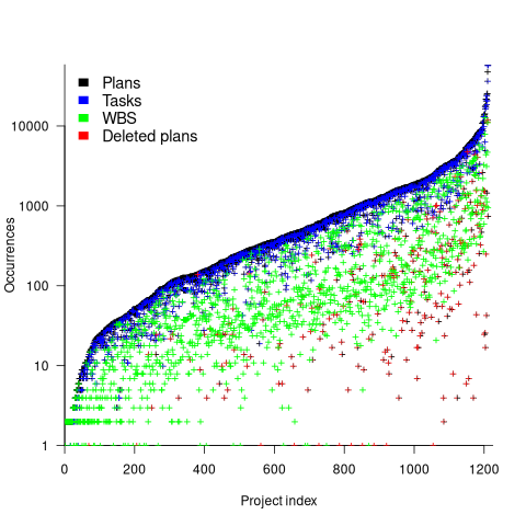
The average ratio of  is 8.4 (standard deviation 23). An exponential or power law (not Weibull) can be fitted to portions of the distribution of project sizes, measured in number of plans or tasks. If project size really does follow a single common distribution, a much larger sample size will be needed to reliably fit it.
The plot below shows, for each project (sorted by total person hours, in red), the number of elapsed days from start of first to end of last task (green), and number of people who worked on at least one task (blue) (projects implemented by a single person do not have consistent time data; code+data):
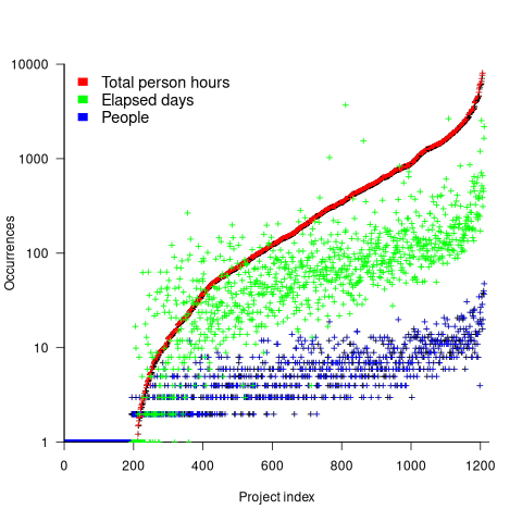
For a given number of person hours worked on a project, there is an order of magnitude variation in elapsed days and number of people who worked on at least one task.
This dataset contains a huge amount of detail, and I’m sure there are lots of patterns to be found. But, what are the important questions to ask, that would be useful to project managers. When I ask managers what project questions they would like answers, the response is often one of quizzical uncertainty. There are plenty of people promoting their opinions, and it’s very rare to encounter anybody asking meaningful questions.
Remotivating data analysed for another purpose
The motivation for fitting a regression model has a major impact on the model created. Some of the motivations include:
- practicing software developers/managers wanting to use information from previous work to help solve a current problem,
- researchers wanting to get their work published seeks to build a regression model that show they have discovered something worthy of publication,
- recent graduates looking to apply what they have learned to some data they have acquired,
- researchers wanting to understand the processes that produced the data, e.g., the author of this blog.
The analysis in the paper: An Empirical Study on Software Test Effort Estimation for Defense Projects by E. Cibir and T. E. Ayyildiz, provides a good example of how different motivations can produce different regression models. Note: I don’t know and have not been in contact with the authors of this paper.
I often remotivate data from a research paper. Most of the data in my Evidence-based Software Engineering book is remotivated. What a remotivation often lacks is access to the original developers/managers (this is often also true for the authors of the original paper). A complicated looking situation is often simplified by background knowledge that never got written down.
The following table shows the data appearing in the paper, which came from 15 projects implemented by a defense industry company certified at CMMI Level-3.
Proj  Test    Req   Test Meetings Faulty    Actual Scenarios
      Plan    Rev   Env          Scenarios  Effort
      Time          Time
P1    144.5  1.006    85     60     100      2850    270
P2     25.5  1.001    25.5    4       5       250     40
P3     68    1.005    42.5   32      65      1966    185
P4     85    1.002    85    104     150      3750    195
P5    198    1.007   123     87     110      3854    410
P6     57    1.006    35     25      20       903    100
P7    115    1.003    92     55      56      2143    225
P8     81    1.009   156     62      72      1988    287
P9    388    1.004   150    208     553     13246   1153
P10   177    1.008    93     77     157      4012    360
P11    62    1.001   175    186     199      5017    310
P12   111    1.005   116     82     143      3994    423
P13    63    1.009   188    177     151      3914    226
P14    32    1.008    25     28       6       435     63
P15 167 1.001 177 143 510 11555 1133 |
where: TestPlanTime is the test plan creation time in hours, ReqRev is the test/requirements review of period in hours, TestEnvTime is the test environment creation time in hours, Meetings is the number of meetings, FaultyScenarios is the number of faulty test scenarios, Scenarios is the number of Scenarios, and ActualEffort is the actual software test effort.
Industrial data is hard to obtain, so well done to the authors for obtaining this data and making it public. The authors fitted a regression model to estimate software test effort, and the model that almost perfectly fits to actual effort is:
ActualEffort=3190 + 2.65*TestPlanTime
            -3170*ReqRevPeriod - 3.5*TestEnvTime
+10.6*Meetings + 11.6*FaultScrenarios + 3.6*Scenarios |
My reading of this model is that having obtained the data, the authors felt the need to use all of it. I have been there and done that.
Why all those multiplication factors, you ask. Isn’t ActualTime simply the sum of all the work done? Yes it is, but the above table lists the work recorded, not the work done. The good news is that the fitted regression models shows that there is a very high correlation between the work done and the work recorded.
Is there a simpler model that can be used to explain/predict actual time?
Looking at the range of values in each column, ReqRev varies by just under 1%. Fitting a model that does not include this variable, we get (a slightly less perfect fit):
ActualEffort=100  + 2.0*TestPlanTime
                              - 4.3*TestEnvTime
+10.7*Meetings + 12.4*FaultScrenarios + 3.5*Scenarios |
Simple plots can often highlight patterns present in a dataset. The plot below shows every column plotted against every other column (code+data):

Points forming a straight line indicate a strong correlation, and the points in the top-right ActualEffort/FaultScrenarios plot look straight. In fact, this one variable dominates the others, and fits a model that explains over 99% of the deviation in the data:
ActualEffort=550 + 22.5*FaultScrenarios |
Many of the points in the ActualEffort/Screnarios plot are on a line, and adding Meetings data to the model explains just under 99% of the variance in the data:
actualEffort=-529.5
+15.6*Meetings + 8.7*Scenarios |
Given that FaultScrenarios is a subset of Screnarios, this connectedness is not surprising. Does the number of meetings correlate with the number of new FaultScrenarios that are discovered? Questions like this can only be answered by the original developers/managers.
The original data/analysis was interesting enough to get a paper published. Is it of interest to practicing software developers/managers?
In a small company, those involved are likely to already know what these fitted models are telling them. In a large company, the left hand does not always know what the right hand is doing. A CMMI Level-3 certified defense company is unlikely to be small, so this analysis may be of interest to some of its developer/managers.
A usable estimation model is one that only relies on information available when the estimation is needed. The above models all rely on information that only becomes available, with any accuracy, way after the estimate is needed. As such, they are not practical prediction models.
Agile and Waterfall as community norms
While rapidly evolving computer hardware has been a topic of frequent public discussion since the first electronic computer, it has taken over 40 years for the issue of rapidly evolving customer requirements to become a frequent topic of public discussion (thanks to the Internet).
The following quote is from the Opening Address, by Andrew Booth, of the 1959 Working Conference on Automatic Programming of Digital Computers (published as the first “Annual Review in Automatic Programming”):
'Users do not know what they wish to do.' This is a profound truth. Anyone who has had the running of a computing machine, and, especially, the running of such a machine when machines were rare and computing time was of extreme value, will know, with exasperation, of the user who presents a likely problem and who, after a considerable time both of machine and of programmer, is presented with an answer. He then either has lost interest in the problem altogether, or alternatively has decided that he wants something else. |
Why did the issue of evolving customer requirements lurk in the shadows for so long?
Some of the reasons include:
- established production techniques were applied to the process of building software systems. What is now known in software circles as the Waterfall model was/is an established technique. The figure below is from the 1956 paper Production of Large Computer Programs by Herbert Benington (Winston Royce’s 1970 paper has become known as the paper that introduced Waterfall, but the contents actually propose adding iterations to what Royce treats as an established process):
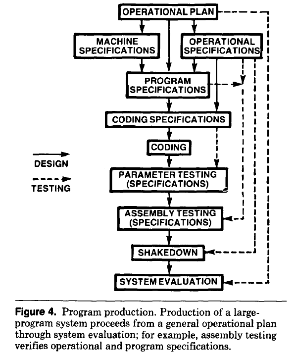
- management do not appreciate how quickly requirements can change (at least until they have experience of application development). In the 1980s, when microcomputers were first being adopted by businesses, I had many conversations with domain experts who were novice programmers building their first application for their business/customers. They were invariably surprised by the rate at which requirements changed, as development progressed.
While in public the issue lurked in the shadows, my experience is that projects claiming to be using Waterfall invariably had back-channel iterations, and requirements were traded, i.e., drop those and add these. Pre-Internet, any schedule involving more than two releases a year could be claimed to be making frequent releases.
Managers claimed to be using Waterfall because it was what everybody else did (yes, some used it because it was the most effective technique for their situation, and on some new projects it may still be the most effective technique).
Now that the issue of rapidly evolving requirements is out of the closet, what’s to stop Agile, in some form, being widely used when ‘rapidly evolving’ needs to be handled?
Discussion around Agile focuses on customers and developers, with middle management not getting much of a look-in. Companies using Agile don’t have many layers of management. Switching to Agile results in a lot of power shifting from middle management to development teams, in fact, these middle managers now look surplus to requirements. No manager is going to support switching to a development approach that makes them redundant.
Adam Yuret has another theory for why Agile won’t spread within enterprises. Making developers the arbiters of maximizing customer value prevents executives mandating new product features that further their own agenda, e.g., adding features that their boss likes, but have little customer demand.
The management incentives against using Agile in practice does not prevent claims being made about using Agile.
Now that Agile is what everybody claims to be using, managers who don’t want to stand out from the crowd find a way of being part of the community.
How much productive work does a developer do?
Measuring develop productivity is a nightmare issue that I do my best to avoid.
Study after study has found that workers organise their work to suit themselves. Why should software developers be any different?
Studies of worker performance invariably find that the rate of work is higher when workers are being watched by researchers/managers; this behavior is known as the Hawthorne effect. These studies invariably involve some form of production line work involving repetitive activities. Time is a performance metric that is easy to measure for repetitive activities, and directly relatable to management interests.
A study by Bernstein found that production line workers slowed down when observed by management. On the production line studied, it was not possible to get the work done in the allotted time using the management prescribed techniques, so workers found more efficient techniques that were used when management were not watching.
I have worked on projects where senior management decreed that development was to be done according to some latest project management technique. Developers quickly found that the decreed technique was preventing work being completed on time, so ignored it while keeping up a facade to keep management happy (who appeared to be well aware of what was going on). Other developers have told me of similar experiences.
Studies of software developer performance often implicitly assume that whatever the workers (i.e., developers) say must be so; there is no thought given to the possibility that the workers are promoting work processes that suits their interests and not managements.
Just like workers in other industries, software developers can be lazy, lack interest in doing a good job, unprofessional, a slacker, etc.
Hard-working, diligent developers can be just as likely as the slackers, to organise work to suit themselves. A good example of this is adding product features that the developer wants to add, rather than features that the customer wants to use, or working on features/performance that exceed the original requirements (known as gold plating in other industries).
Developers will lobby for projects to use the latest language/package/GUI/tools in their work. While issues around customer/employer cost/benefit might be cited as a consideration, evidence, in the form of a cost/benefit analysis, is not usually given.
Like most people, developers want others to have a good opinion of them. As writers, of code, developers can attach a lot of weight to how its quality will be perceived by other developer. One consequence of this is a willingness to regularly spend time polishing good-enough code. An economic cost/benefit of refactoring is rarely a consideration.
The first step of finding out if developers are doing productive work is finding out what they are doing, or even better, planning in some detail what they should be doing.
Developers are not alone in disliking having their activities constrained by detailed plans. Detailed plans imply some form of estimates, and people really hate making estimates.
My view of the rationale for estimating in story points (i.e., monopoly money) is that they relieve the major developer pushback on estimating, while allowing management to continue to create short-term (e.g., two weeks) plans. The assumption made is that the existence of detailed plans reduces worker wiggle-room for engaging in self-interest work.
Analysis of when refactoring becomes cost-effective
In a cost/benefit analysis of deciding when to refactor code, which variables are needed to calculate a good enough result?
This analysis compares the excess time-code of future work against the time-cost of refactoring the code. Refactoring is cost-effective when the reduction in future work time is less than the time spent refactoring. The analysis finds a relationship between work/refactoring time-costs and number of future coding sessions.
Linear, or supra-linear case
Let’s assume that the time needed to write new code grows at a linear, or supra-linear rate, as the amount of code increases ( ):
):

where:  is the base time for writing new code on a freshly refactored code base,
  is the number of lines of code that have been written since the last refactoring, and
  and
and  are constants to be decided.
The total time spent writing code over  sessions is:
^x}")
If the same number of new lines is added in every coding session,  , and is an integer constant, then the sum has a known closed form, e.g.:
x=1, ^1}={n(n+1)}/2L_s") ; x=2,
; x=2, ^2}={n(n+1)(2n+1)}/6{L_s}^2")
Let’s assume that the time taken to refactor the code written after sessions is:
^y")
where:  and
and  are constants to be decided.
The reason for refactoring is to reduce the time-cost of subsequent work; if there are no subsequent coding sessions, there is no economic reason to refactor the code. If we assume that after refactoring, the time taken to write new code is reduced to the base cost, , and that we believe that coding will continue at the same rate for at least another  sessions, then refactoring existing code after sessions is cost-effective when:
^y < k_1sum{i=n+1}{n+f}{(iL_s)^x}")
assuming that is much smaller than , setting  , and rearranging we get:

after rearranging we obtain a lower limit on the number of future coding sessions, , that must be completed for refactoring to be cost-effective after session ::

It is expected that  ; the contribution of code size, at the end of every session, in the calculation of
  and
and  is equal (i.e.,
 ^y") ), and the overhead of adding new code is very unlikely to be less than refactoring all the newly written code.
), and the overhead of adding new code is very unlikely to be less than refactoring all the newly written code.
With  ,
,  must be close to zero; otherwise, the likely relatively large value of (e.g., 100+) would produce surprisingly high values of .
Sublinear case
What if the time overhead of writing new code grows at a sublinear rate, as the amount of code increases?
Various attributes have been found to strongly correlate with the  of lines of code. In this case, the expressions for and become:

")
and the cost/benefit relationship becomes:
 < k_1sum{i=n+1}{n+f}{log(iL_s)}")
applying Stirling’s approximation and simplifying (see Exact equations for sums at end of post for details) we get:
 < k_1(f(log(n+f)-1)+f log{L_s})")
+log{L_s}-1} < f")
applying the series expansion (for  ):
):  , we get
 < f")
Discussion
What does this analysis of the cost/benefit relationship show that was not obvious (i.e., the relationship  is obviously true)?
What the analysis shows is that when real-world values are plugged into the full equations, all but two factors have a relatively small impact on the result.
A factor not included in the analysis is that source code has a half-life (i.e., code is deleted during development), and the amount of code existing after sessions is likely to be less than the  used in the analysis (see Agile analysis).
As a project nears completion, the likelihood of there being more coding sessions decreases; there is also the every present possibility that the project is shutdown.
The values of and encode information on the skill of the developer, the difficulty of writing code in the application domain, and other factors.
Exact equations for sums
The equations for the exact sums, for  , are:
")
+1)")
(2n(n+1)+2fn+f+f^2)")
-zeta(-0.5, f+n+1)") , where
, where  is the Hurwitz zeta function.
Sum of a log series: !}/{n!}}+f log{L_s}")
using Stirling’s approximation we get
!)}-log(n!) approx (n+f-0.5)log(n+f)-(n+f)-((n-0.5)log n-n)")
simplifying
!)}-log(n!) approx (n-0.5)log(1+f/n)+f log(n+f)-f")
and assuming that is much smaller than gives
!)}-log(n!) approx f(log(n+f)-1)")
Update
The analysis above assumes that the time contribution of the base rate, , is independent of the changes,  . The following analysis combines these two contributions into a single rate:
L)^b}")
where:  ,
,  , , and are positive constants, with
  , and
, and  .
.
The following is a very good approximation to this sum (thanks to Grok 4.1 beta; chat script):
L})")
where: L")
Software engineering as a hedonistic activity
My discussions with both managers and developers on software development processes invariably end up on the topic of developer happiness. Managers want to keep their development teams happy, and there is a longstanding developer culture of entitlement to work that they find interesting.
Companies in general want to keep their employees happy, irrespective of the kind of work they do. What makes developers different, from management’s perspective, is that demand for good software developers far outstrips supply.
Many developers approach software engineering as a hedonistic activity; yes, there are those who only do it for the money.
The huge quantity of open source software, much of it written out of personal interest rather than paid employment, provides evidence for there being many people willing to create software because of the pleasure they get from doing it.
Software developers only get to indulge in hedonistic development activities (e.g., choosing which tools to use, how to structure their code, and not having to provide estimates) because of the relative ease with which competent developers can obtain another job. Replacing developers is time-consuming and expensive, which gives existing employees a lot of bargaining power with management.
Some of the consequences of managements’ desire to keep developers happy, or at least not unhappy include:
- Not pushing too hard for an estimate of the likely time needed to complete a task,
- giving developers a lot of say in which languages/tools/packages they use. This creates a downstream need to support a wider variety of development ecosystems than might otherwise have been necessary, and further siloing development teams,
- allowing developers to spend time beautifying their code to meet personal opinions about the visual appearance of source.
The balance of power that facilitates hedonism driven development is determined by the relative size of the employment market in the supply and demand for software developers. Once demand falls below the available supply, finding a new job becomes more difficult, shifting the balance of power away from developers to managers.
I am not expecting supply to exceed demand any time soon. While International computer companies have been laying off lots of staff, demand from small companies appears to be strong (based on the ever-present ‘We’re hiring’ slides I regularly see at London meetups), but things may change. Tools such as ChatGPT are far from good enough to replace developers in the near term.
Career progression: an invisible issue in software development
Career progression is an important issue in the development of some software systems, but its impact is rarely discussed, let along researched. A common consequence of career progression is that a project looses a member of staff, e.g., they move to work on a different project, or leave the company. Hiring staff and promoting staff are related neglected research areas.
Understanding the initial and ongoing development of non-trivial software systems requires an understanding of the career progression, and expectations of progression, of the people working on the system.
Effectively working on a software system requires some amount of knowledge of how it operates, or is intended to operate. The loss of a person with working knowledge of a system reduces the rate at which a project can be further developed. It takes time to find a suitable replacement, and for that person’s knowledge of the behavior of the existing system to reach a workable level.
We know that most software is short-lived, but know almost nothing about the involvement-lifetime of those who work on software systems.
There has been some research studying the durations over which people have been involved with individual Open source projects. However, I don’t believe the findings from this research, because I think that non-paid involvement on an Open source project has very different duration and motivation characteristics than a paying job (there are also data cleaning issues around the same person using multiple email addresses, and people working in small groups with one person submitting code).
Detailed employment data, in bulk, has commercial value, and so is rarely freely available. It is possible to scrape data from the adverts of job websites, but this only provides information about the kinds of jobs available, not the people employed.
LinkedIn contains lots of detailed employment history, and the US courts have ruled that it is not illegal to scrape this data. It’s on my list of things to do, and I keep an eye out for others making such data available.
The National Longitudinal Survey of Youth has followed the lives of 10k+ people since 1979 (people were asked to detail their lives in periodic surveys). Using this data, Joseph, Boh, Ang, and Slaughter investigated the job categories within the career paths of 500 people who had worked in a technical IT role. The plot below shows the career paths of people who had spent at least five years working in an IT role (code+data):
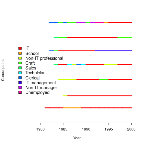
Employment history provides an upper bound for the time that a person is likely to have worked on a project (being employed to work on an Open source project while, over time, working at multiple companies is an edge case).
A company may have employees simultaneously working on multiple projects, spending a percentage of their time on each. How big a resource impact is the loss of such a person? Were they simply the same kind of cog in multiple projects, or did they play an important synchronization role across projects? Details on all the projects a person worked on would help answer some questions.
Building a software system involves a lot more than writing the code. Technical managers working on high level, broad brush, issues. The project knowledge that technical managers have contributes to ongoing work, and the impact of loosing a technical manager is probably more of a longer term issue than loosing a coding-developer.
There are systems that are developed and maintained by essentially one person over many years. These get written about and celebrated, but are comparatively rare.
One of the more reliable ways of estimating developer productivity is to measure the impact of them leaving a project.
Evaluating estimation performance
What is the best way to evaluate the accuracy of an estimation technique, given that the actual values are known?
Estimates are often given as point values, and accuracy scoring functions (for a sequence of estimates) have the form }") , where is the number of estimated values,
, where is the number of estimated values,  the estimates, and
  the actual values; smaller
  is better.
Commonly used scoring functions include:
=(E-A)^2") , known as squared error (SE)
, known as squared error (SE)=delim{|}{E-A}{|}") , known as absolute error (AE)
, known as absolute error (AE)=delim{|}{E-A}{|}/A") , known as absolute percentage error (APE)
, known as absolute percentage error (APE)=delim{|}{E-A}{|}/E") , known as relative error (RE)
, known as relative error (RE)
APE and RE are special cases of: =delim{|}{1-(A/E)^{beta}}{|}") , with
, with  and
and  respectively.
Let’s compare three techniques for estimating the time needed to implement some tasks, using these four functions.
Assume that the mean time taken to implement previous project tasks is known,  . When asked to implement a new task, an optimist might estimate 20% lower than the mean,
  , while a pessimist might estimate 20% higher than the mean,
  . Data shows that the distribution of the number of tasks taking a given amount of time to implement is skewed, looking something like one of the lines in the plot below (code):
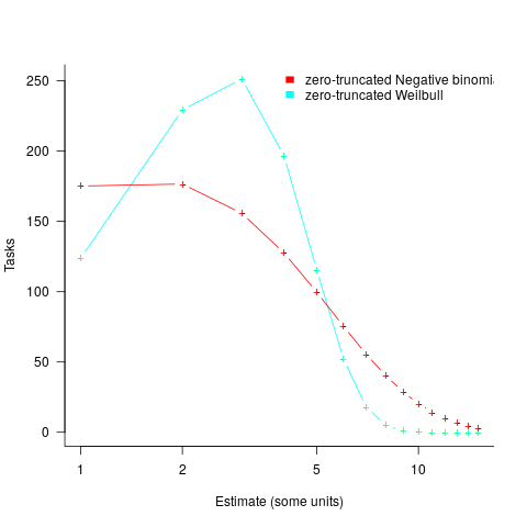
We can simulate task implementation time by randomly drawing values from a distribution having this shape, e.g., zero-truncated Negative binomial or zero-truncated Weibull. The values of  and
and  are calculated from the mean, , of the distribution used (see code for details). Below is each estimator’s score for each of the scoring functions (the best performing estimator for each scoring function in bold; 10,000 values were used to reduce small sample effects):
    SE   AE   APE   RE

  2.73 1.29 0.51 0.56

 2.31 1.23 0.39 0.68

  2.70 1.37 0.36 0.86
Surprisingly, the identity of the best performing estimator (i.e., optimist, mean, or pessimist) depends on the scoring function used. What is going on?
The analysis of scoring functions is very new. A 2010 paper by Gneiting showed that it does not make sense to select the scoring function after the estimates have been made (he uses the term forecasts). The scoring function needs to be known in advance, to allow an estimator to tune their responses to minimise the value that will be calculated to evaluate performance.
The mathematics involves Bregman functions (new to me), which provide a measure of distance between two points, where the points are interpreted as probability distributions.
Which, if any, of these scoring functions should be used to evaluate the accuracy of software estimates?
In software estimation, perhaps the two most commonly used scoring functions are APE and RE. If management selects one or the other as the scoring function to rate developer estimation performance, what estimation technique should employees use to deliver the best performance?
Assuming that information is available on the actual time taken to implement previous project tasks, then we can work out the distribution of actual times. Assuming this distribution does not change, we can calculate APE and RE for various estimation techniques; picking the technique that produces the lowest score.
Let’s assume that the distribution of actual times is zero-truncated Negative binomial in one project and zero-truncated Weibull in another (purely for convenience of analysis, reality is likely to be more complicated). Management has chosen either APE or RE as the scoring function, and it is now up to team members to decide the estimation technique they are going to use, with the aim of optimising their estimation performance evaluation.
A developer seeking to minimise the effort invested in estimating could specify the same value for every estimate. Knowing the scoring function (top row) and the distribution of actual implementation times (first column), the minimum effort developer would always give the estimate that is a multiple of the known mean actual times using the multiplier value listed:
                   APE   RE

Negative binomial  1.4   0.5

Weibull            1.2   0.6
For instance, management specifies APE, and previous task/actuals has a Weibull distribution, then always estimate the value  .
.
What mean multiplier should Esta Pert, an expert estimator aim for? Esta’s estimates can be modelled by the equation ") , i.e., the actual implementation time multiplied by a random value uniformly distributed between 0.5 and 2.0, i.e., Esta is an unbiased estimator. Esta’s table of multipliers is:
, i.e., the actual implementation time multiplied by a random value uniformly distributed between 0.5 and 2.0, i.e., Esta is an unbiased estimator. Esta’s table of multipliers is:
                   APE     RE

Negative binomial  1.0   0.7

Weibull                     1.0     0.7
A company wanting to win contracts by underbidding the competition could evaluate Esta’s performance using the RE scoring function (to motivate her to estimate low), or they could use APE and multiply her answers by some fraction.
In many cases, developers are biased estimators, i.e., individuals consistently either under or over estimate. How does an implicit bias (i.e., something a person does unconsciously) change the multiplier they should consciously aim for (having analysed their own performance to learn their personal percentage bias)?
The following table shows the impact of particular under and over estimate factors on multipliers:
                 0.8 underestimate bias   1.2 overestimate bias

Score function          APE   RE            APE   RE

Negative binomial        1.3   0.9           0.8   0.6

Weibull                 1.3       0.9           0.8   0.6
Let’s say that one-third of those on a team underestimate, one-third overestimate, and the rest show no bias. What scoring function should a company use to motivate the best overall team performance?
The following table shows that neither of the scoring functions motivate team members to aim for the actual value when the distribution is Negative binomial:
                    APE      RE

Negative binomial    1.1     0.7

Weibull                               1.0       0.7
One solution is to create a bespoke scoring function for this case. Both APE and RE are special cases of a more general scoring function (see top). Setting  in this general form creates a scoring function that produces a multiplication factor of 1 for the Negative binomial case.
NoEstimates panders to mismanagement and developer insecurity
Why do so few software development teams regularly attempt to estimate the duration of the feature/task/functionality they are going to implement?
Developers hate giving estimates; estimating is very hard and estimates are often inaccurate (at a minimum making the estimator feel uncomfortable and worse when management treats an estimate as a quotation). The future is uncertain and estimating provides guidance.
Managers tell me that the fear of losing good developers dissuades them from requiring teams to make estimates. Developers have told them that they would leave a company that required them to regularly make estimates.
For most of the last 70 years, demand for software developers has outstripped supply. Consequently, management has to pay a lot more attention to the views of software developers than the views of those employed in most other roles (at least if they want to keep the good developers, i.e., those who will have no problem finding another job).
It is not difficult for developers to get a general idea of how their salary, working conditions and practices compares with other developers in their field/geographic region. They know that estimating is not a common practice, and unless the economy is in recession, finding a new job that does not require estimation could be straight forward.
Management’s demands for estimates has led to the creation of various methods for calculating proxy estimate values, none of which using time as the unit of measure, e.g., Function points and Story points. These methods break the requirements down into smaller units, and subcomponents from these units are used to calculate a value, e.g., the Function point calculation includes items such as number of user inputs and outputs, and number of files.
How accurate are these proxy values, compared to time estimates?
As always, software engineering data is sparse. One analysis of 149 projects found that  , with the variance being similar to that found when time was estimated. An analysis of Function point calculation data found a high degree of consistency in the calculations made by different people (various Function point organizations have certification schemes that require some degree of proficiency to pass).
Managers don’t seem to be interested in comparing estimated Story points against estimated time, preferring instead to track the rate at which Story points are implemented, e.g., velocity, or burndown. There are tiny amounts of data comparing Story points with time and Function points.
The available evidence suggests a relationship connecting Function points to actual time, and that Function points have similar error bounds to time estimates; the lack of data means that Story points are currently just a source of technobabble and number porn for management power-points (send me Story point data to help change this situation).
Multiple estimates for the same project
The first question I ask, whenever somebody tells me that a project was delivered on schedule (or within budget), is which schedule (or budget)?
New schedules are produced for projects that are behind schedule, and costs get re-estimated.
What patterns of behavior might be expected to appear in a project’s reschedulings?
It is to be expected that as a project progresses, subsequent schedules become successively more accurate (in the sense of having a completion date and cost that is closer to the final values). The term cone of uncertainty is sometimes applied as a visual metaphor in project management, with the schedule becoming less uncertain as the project progresses.
The only publicly available software project rescheduling data, from Landmark Graphics, is for completed projects, i.e., cancelled projects are not included (121 completed projects and 882 estimates).
The traditional project management slide has some accuracy metric improving as work on a project approaches completion. The plot below shows the percentage of a project completed when each estimate is made, against the ratio  ; the y-axis uses a log scale so that under/over estimates appear symmetrical (code+data):
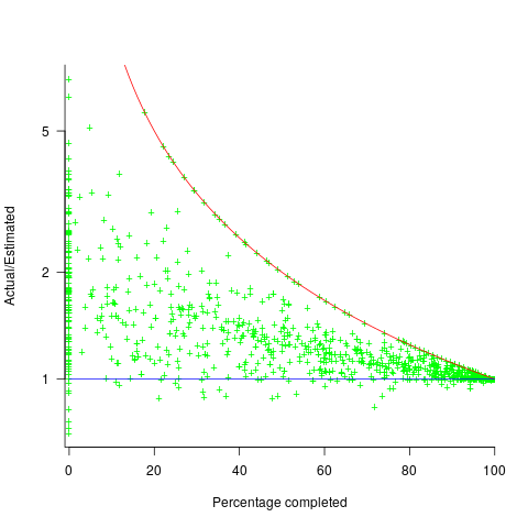
The closer a point to the blue line, the more accurate the estimate. The red line shows maximum underestimation, i.e., estimating that the project is complete when there is still more work to be done. A new estimate must be greater than (or equal) to the work already done, i.e.,  , and
, and  .
.
Rearranging, we get:  (plotted in red). The top of the ‘cone’ does not represent managements’ increasing certainty, with project progress, it represents the mathematical upper bound on the possible inaccuracy of an estimate.
In theory there is no limit on overestimating (i.e., points appearing below the blue line), but in practice management are under pressure to deliver as early as possible and to minimise costs. If management believe they have overestimated, they have an incentive to hang onto the time/money allocated (the future is uncertain).
Why does management invest time creating a new schedule?
If information about schedule slippage leaks out, project management looks bad, which creates an incentive to delay rescheduling for as long as possible (i.e., let’s pretend everything will turn out as planned). The Landmark Graphics data comes from an environment where management made weekly reports and estimates were updated whenever the core teams reached consensus (project average was eight times).
The longer a project is being worked on, the greater the opportunity for more unknowns to be discovered and the schedule to slip, i.e., longer projects are expected to acquire more re-estimates. The plot below shows the number of estimates made, for each project, against the initial estimated duration (red/green) and the actual duration (blue/purple); lines are loess fits (code+data):
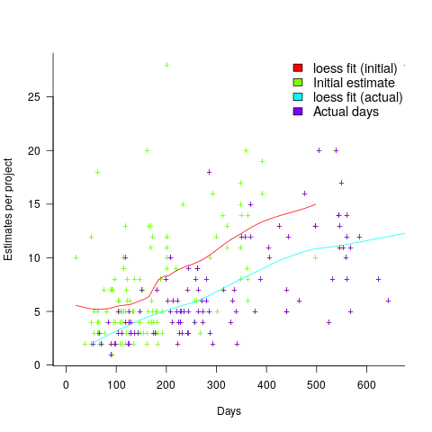
What might be learned from any patterns appearing in this data?
When presented with data on the sequence of project estimates, my questions revolve around the reasons for spending time creating a new estimate, and the amount of time spent on the estimate.
A lot of time may have been invested in the original estimate, but how much time is invested in subsequent estimates? Are later estimates simply calculated as a percentage increase, a politically acceptable value (to the stakeholder funding for the project), or do they take into account what has been learned so far?
The information needed to answer these answers is not present in the data provided.
However, this evidence of the consistent provision of multiple project estimates drives another nail in to the coffin of estimation research based on project totals (e.g., if data on project estimates is provided, one estimate per project, were all estimates made during the same phase of the project?)
Recent Comments