Archive
Multiple estimates for the same project
The first question I ask, whenever somebody tells me that a project was delivered on schedule (or within budget), is which schedule (or budget)?
New schedules are produced for projects that are behind schedule, and costs get re-estimated.
What patterns of behavior might be expected to appear in a project’s reschedulings?
It is to be expected that as a project progresses, subsequent schedules become successively more accurate (in the sense of having a completion date and cost that is closer to the final values). The term cone of uncertainty is sometimes applied as a visual metaphor in project management, with the schedule becoming less uncertain as the project progresses.
The only publicly available software project rescheduling data, from Landmark Graphics, is for completed projects, i.e., cancelled projects are not included (121 completed projects and 882 estimates).
The traditional project management slide has some accuracy metric improving as work on a project approaches completion. The plot below shows the percentage of a project completed when each estimate is made, against the ratio  ; the y-axis uses a log scale so that under/over estimates appear symmetrical (code+data):
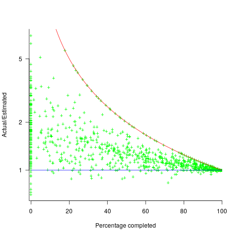
The closer a point to the blue line, the more accurate the estimate. The red line shows maximum underestimation, i.e., estimating that the project is complete when there is still more work to be done. A new estimate must be greater than (or equal) to the work already done, i.e.,  , and
, and  .
.
Rearranging, we get:  (plotted in red). The top of the ‘cone’ does not represent managements’ increasing certainty, with project progress, it represents the mathematical upper bound on the possible inaccuracy of an estimate.
In theory there is no limit on overestimating (i.e., points appearing below the blue line), but in practice management are under pressure to deliver as early as possible and to minimise costs. If management believe they have overestimated, they have an incentive to hang onto the time/money allocated (the future is uncertain).
Why does management invest time creating a new schedule?
If information about schedule slippage leaks out, project management looks bad, which creates an incentive to delay rescheduling for as long as possible (i.e., let’s pretend everything will turn out as planned). The Landmark Graphics data comes from an environment where management made weekly reports and estimates were updated whenever the core teams reached consensus (project average was eight times).
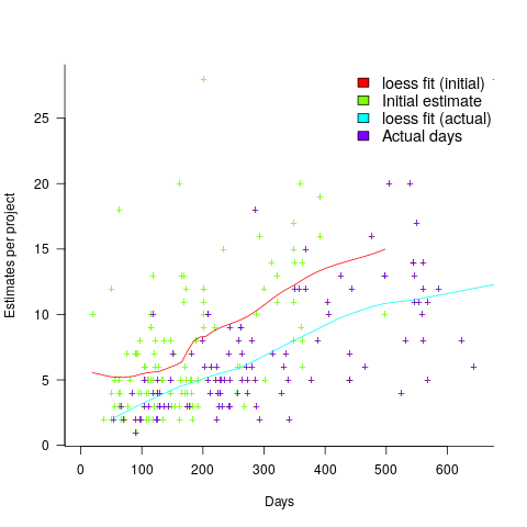
The longer a project is being worked on, the greater the opportunity for more unknowns to be discovered and the schedule to slip, i.e., longer projects are expected to acquire more re-estimates. The plot below shows the number of estimates made, for each project, against the initial estimated duration (red/green) and the actual duration (blue/purple); lines are loess fits (code+data):
What might be learned from any patterns appearing in this data?
When presented with data on the sequence of project estimates, my questions revolve around the reasons for spending time creating a new estimate, and the amount of time spent on the estimate.
A lot of time may have been invested in the original estimate, but how much time is invested in subsequent estimates? Are later estimates simply calculated as a percentage increase, a politically acceptable value (to the stakeholder funding for the project), or do they take into account what has been learned so far?
The information needed to answer these answers is not present in the data provided.
However, this evidence of the consistent provision of multiple project estimates drives another nail in to the coffin of estimation research based on project totals (e.g., if data on project estimates is provided, one estimate per project, were all estimates made during the same phase of the project?)
Readability: a scientific approach
Readability, as applied to software development today, is a meaningless marketing term. Readability is promoted as a desirable attribute, and is commonly claimed for favored programming languages, particular styles of programming, or ways of laying out source code.
Whenever somebody I’m talking to, or listening to in a talk, makes a readability claim, I ask what they mean by readability, and how they measured it. The speaker invariably fumbles around for something to say, with some dodging and weaving before admitting that they have not measured readability. There have been a few studies that asked students to rate the readability of source code (no guidance was given about what readability might be).
If somebody wanted to investigate readability from a scientific perspective, how might they go about it?
The best way to make immediate progress is to build on what is already known. There has been over a century of research on eye movement during reading, and two model of eye movement now dominate, i.e., the E-Z Reader model and SWIFT model. Using eye-tracking to study developers is slowly starting to be adopted by researchers.
Our eyes don’t smoothly scan the world in front of us, rather they jump from point to point (these jumps are known as a saccade), remaining fixed long enough to acquire information and calculate where to jump next. The image below is an example from an eye tracking study, where subjects were asking to read a sentence (see figure 770.11). Each red dot appears below the center of each saccade, and the numbers show the fixation time (in milliseconds) for that point (code):

Models of reading are judged by the accuracy of their predictions of saccade landing points (within a given line of text), and fixation time between saccades. Simulators implementing the E-Z Reader and SWIFT models have found that these models have comparable performance, and the robustness of these models are compared by looking at the predictions they make about saccade behavior when reading what might be called unconventional material, e.g., mirrored or scarmbeld text.
What is the connection between the saccades made by readers and their understanding of what they are reading?
Studies have found that fixation duration increases with text difficulty (it is also affected by decreases with word frequency and word predictability).
It has been said that attention is the window through which we perceive the world, and our attention directs what we look at.
A recent study of the SWIFT model found that its predictions of saccade behavior, when reading mirrored or inverted text, agreed well with subject behavior.
I wonder what behavior SWIFT would predict for developers reading a line of code where the identifiers were written in camelCase or using underscores (sometimes known as snake_case)?
If the SWIFT predictions agreed with developer saccade behavior, a raft of further ‘readability’ tests spring to mind. If the SWIFT predictions did not agree with developer behavior, how might the model be updated to support the reading of lines of code?
Until recently, the few researchers using eye tracking to investigate software engineering behavior seemed to be having fun playing with their new toys. Things are starting to settle down, with some researchers starting to pay attention to existing models of reading.
What do I predict will be discovered?
Lots of studies have found that given enough practice, people can become proficient at handling some apparently incomprehensible text layouts. I predict that given enough practice, developers can become equally proficient at most of the code layout schemes that have been proposed.
The important question concerning text layout, is: which one enables an acceptable performance from a wide variety of developers who have had little exposure to it? I suspect the answer will be the one that is closest to the layout they have had the most experience,i.e., prose text.
Cognitive bias or not paying enough attention?
Assume you are responsible for two teams who independently work on projects, say Team A and Team B. The teams have different work completion rates, with Team A completing work at the rate of 70 widgets per week, while Team B completes 30 widgets per week. Both teams always work on projects that require the completion of the same number of widgets.
You have the resources to send just one of the teams on a course. It is predicted that sending Team A on the course would improve their performance to 110 widgets per week, while attending the course would improve the performance of Team B to 40 widgets per week.
Senior management have decreed that time to market is the metric by which project managers are judged.
You want to impress senior management by significantly improving time to market for your projects; which team do you send on the course (i.e., the one that is likely to experience the largest reduction in time to market)?
This question is a restatement of a one involving cars travelling at different speeds, that has grown into a niche research area. Studies have found that a large percentage of subjects give the wrong answer, and they are said to have a time-saving bias, or time-loss bias.
The inability to correctly process “inverse variables” has been given as the reason people tend to give the wrong answer. The term “inverse variables” comes from the formula for calculating completion time, where the velocity appears as the denominator. Another way of looking at this problem is that when going slowly, there is more scope for improvement, compared to when going much faster.
A speed increase from 30 to 40 is only 10, or a 33% improvement; while an increase from 70 to 110 is an increase of 40, or 57%. Based on these numbers, Team A should be sent on the course.
However, we are interested in time to market. Let’s assume that both teams have to complete a project requiring 100 widgets. Before attending the course, Team A completes 100 widgets in 100/70=1.4 weeks, and Team B completes 100 widgets in 100/30=3.3 weeks. After attending the course, Team A would complete 100 widgets in 100/110=0.91 weeks, and Team B would complete 100 widgets in 100/40=2.5 weeks. Time to market for Team A has been reduced by (1.4-0.9)=0.5 weeks, while the reduction for Team B is (3.3-2.5)=0.8 weeks. So sending Team B on the course makes you look better, on the time to market metric.
If somebody ran an experiment with project managers, would the subjects tend to incorrectly process “inverse variables”. Well, somebody has done the experiment, and yes, many subjects exhibited the time-saving bias (the experimental scenario described in the appendix is a lot easier to understand than the one in the main body of the paper, which is a mess; Magne Jørgensen continues to be the only person doing interesting experiments in software estimation).
It has become common practice that, when a large percentage of subjects in a psychology experiment respond in ways that are inconsistent with a mathematical approach, the behavior is labelled as being a bias. I think the use of this terminology makes the behavior sound more interesting than it actually is; what’s wrong with saying that people make mistakes. Perhaps labelling experimental responses as being a bias makes it easier to get papers published.
Whether people are biased, or don’t pay enough attention, when solving non-trivial equations, what might be done about it?
This is not about whether any particular metric is a useful one, rather it is about calculating the right answer for whatever metric happens to be chosen.
Would an awareness campaign highlighting the problems people have with “inverse variables” be worthwhile? I don’t think so. Many people have problems with equations, and I don’t see why this case is more worthy of being highlighted than any other.
Am I missing something?
Psychology researchers are interested in figuring out the functioning of the brain/mind, so they are looking for patterns in the responses subjects give. Once someone has published a few papers on a research topic, they become invested in it. If they continue to get funding, the papers keep on coming. Sometimes a niche topic acquires a major following, and the work contributes to a major change of thinking about the mind, e.g., the Wason selection task helped increase the evidence that culture has an impact on cognitive behavior.
I think that software engineering researchers need to carefully evaluate the likely importance of behaviors that psychology researchers have labelled as a bias.
Actual implementation times are often round numbers
To what extent do developers consciously influence the time taken to actually complete a task?
If the time estimated to complete a task is rather generous, a developer has the opportunity to follow Parkinson’s law (i.e., “work expands so as to fill the time available for its completion”), or if the time is slightly less than appears to be required, they might work harder to finish within the estimated time (like some marathon runners have a target time)?
The use of round numbers are a prominent pattern seen in task estimation times.
If round numbers appeared more often in the actual task completion time than would be expected by chance, it would suggest that developers are sometimes working to a target time. The following plot shows the number of tasks taking a given amount of actual time to complete, for project 615 in the CESAW dataset (similar patterns are present in the actual times of other projects; code+data):
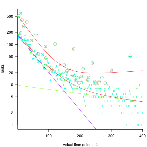
The red lines are a fitted bi-exponential distribution to the ‘spike’ (i.e., round numbers, circled in grey) and non-spike points (spikes automatically selected, see code for details), green and purple lines are the two components of the non-spike fit.
Tasks are not always started and completed in one continuous work session, work may be spread over multiple work sessions; the CESAW data includes the start/end time of every work session associated with each task (85% of tasks involve more than one work session, for project 615). The following plots are based on work sessions, rather than tasks, for tasks worked on over two (left) and three (right) sessions; colored lines denote session ordering within a task (code+data):
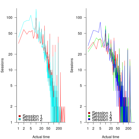
Shorter sessions dominate for the last session of task implementation, and spikes in the counts indicate the use of round numbers in all session positions (e.g., 180 minutes, which may be half a day).
Perhaps round number work session times are a consequence of developers using round number wall-clock times to start and end work sessions. The plot below shows (left) the number of work sessions starting at a given number of minutes past the hour, and (right) the number of work sessions ending at a given number of minutes past the hour; both for project 615 (code+data):

The arrow (green) shows the direction of the mean, and the almost invisible interior line shows that the length of the mean is almost zero. The five-minute points have slightly more session starts/ends than the surrounding minute values, but are more like bumps than spikes. The start of the hour, and 30-minutes, have prominent spikes, which might be caused by the start/end of the working day, and start/end of the lunch break.
Five-minutes is a convenient small rounding interval to either expand implementation time, or to target as a completion time. The following plot shows, for each of the 47 individuals working on project 615, the number of actual session times and the number exactly divisible by five. The green line shows the case where every actual is divisible by five, the purple line where 20% are divisible by five (expected for unbiased timing), the dashed purple lines show one standard deviation, the blue/green line is a fitted regression model ( ) (code+data):
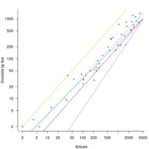
It appears that on average, five-minute session times occur twice as often as expected by chance; two individuals round all their actual session times (ok, it’s not that unlikely for the person with just two sessions).
Does it matter that some developers have a preference for using round numbers when recording time worked?
The use of round numbers in the recording of actual work sessions will inflate the total actual time for most tasks (because most tasks involve more than one session, and assuming that most rounding is not caused by developers striving to meet a target). The amount of error introduced is probably a lot less than the time variability caused by other implementation factors (I have yet to do the calculation).
I see the use of round numbers as a means of unpicking developer work habits.
Given the difficulty of getting developers to record anything, requiring them to record to minute-level accuracy appears at best optimistic. Would you work for a manager that required this level of effort detail (I know there is existing practice in other kinds of jobs)?
What can be learned from studying long gone development practices?
Current ideas about the best way of building a software system are heavily influenced by the ideas that captured the attention of previous generations of developers. Can anything of practical use be learned from studying long gone techniques for building software systems?
During the writing of my software engineering book, I was spending a lot of time researching the development techniques used during the twentieth century, and one day I suddenly realised that this was a waste of time. While early software developers tend to be eulogized today, the reality is that they were mostly people who had little idea what they were doing, who through personal competence of being in the right place at the right time managed to produce something good enough. On the whole, twentieth century software development techniques are only of historical interest. Yes, some timeless development principles were discovered, and these can be integrated into today’s techniques (which may also turn out to be of their-time).
My experience of software development in the late 1970s and 1980s is that there was rarely any connection between what management told the world about the development process, and how those reporting to the manager actually did the development.
If you are a manager in a world where software development is still very new, and you are given the job of managing the development of a software system, how do you go about it? A common approach is to apply the techniques that are already being used to run the manager’s organization. On a regular basis, managers came up with the idea of applying techniques from the science of industrial production (which is still happening today).
In the 1970s and 1980s there were usually very visible job hierarchies, and sharply defined roles. Organizations tended to use their existing job hierarchies and roles to create the structure for their software development employees. For years after I started work as a graduate, managers and secretaries were surprised to see me typing; secretaries typed, men did not type, and women developers fumed when they were treated like secretaries (because they had been seen typing).
The manual workers performed data entry, operated the computer (e.g., mounted tapes, and looked after the printer). The junior staff often started with the job title programmer, or perhaps junior programmer and there might be senior programmers; on paper these people wrote the code to implement the functionality specified by a systems analyst (or just analyst, or business analyst, perhaps with added junior or senior). Analysts did not to write code and programmers only coded what the specification they were given, at least according to management.
Pay level was set by the position in the job hierarchy, with those higher up earning more than those below them, and job titles/roles were also mapped to positions in the hierarchy. This created, in theory, a direct correspondence between pay and job title/role. In practice, organizations wanted to keep their productive employees, and so were flexible about the correspondence between pay and title, e.g., during their annual review some people were more interested in the status provided by a job title, while others wanted more money and did not care about job titles. Add into this mix the fact that pay/title levels rarely matched up between organizations, it soon became obvious to all that software job titles were a charade.
How should the people at the sharp end go about building a software system?
Structured programming was the widely cited technique in the 1970s. Consultants promoted their own variants, with Jackson structured programming being widely known in the UK, with regular courses and consultants offering to train staff. Today, structured programming appears remarkably simplistic, great for writing tiny programs (it has an academic pedigree), but not for anything larger than a thousand lines. Part of its appeal may have been this simplicity, many programs were small (because computer memory was measured in kilobytes) and management often thought that problems were simple (a recurring problem). There were a few adaptations that tried to address larger scale issues, e.g., Warnier/Orr structured programming.
The military were major employers of software developers in the 1960s and 1970s. In the US Work Breakdown Structure was mandated by the DOD for project development (for all projects, not just software), and in the UK we had MASCOT. These mandated development methodologies were created by committees, and have not been experimentally tested to be better/worse than any other approach.
I think the best management technique for successfully developing a software system in the 1970s and 1980s (and perhaps in the following decades), is based on being lucky enough to have a few very capable people, and then providing them with what is needed to get the job done while maintaining the fiction to upper management that the agreed bureaucratic plan is being followed.
There is one technique for producing a software system that rarely gets mentioned: keep paying for development until something good enough is delivered. Given the life-or-death need an organization might have for some software systems, paying what it takes may well have been a prevalent methodology during the early days of major software development.
To answer the question posed at the start of this post. What might be learned from a study of early software development techniques is the need for management to have lots of luck and to be flexible; funding is easier to obtain when managing a life-or-death project.
Recent Comments