Archive
Chinchilla Scaling: A replication using the pdf
The paper Chinchilla Scaling: A replication attempt by Besiroglu, Erdil, Barnett, and You caught my attention. Not only a replication, but on the first page there is the enticing heading of section 2, “Extracting data from Hoffmann et al.’s Figure 4”. Long time readers will know of my interest in extracting data from pdfs and images.
This replication found errors in the original analysis, and I, in turn, found errors in the replication’s data extraction.
Besiroglu et al extracted data from a plot by first converting the pdf to Scalable Vector Graphic (SVG) format, and then processing the SVG file. A quick look at their python code suggested that the process was simpler than extracting directly from an uncompressed pdf file.
Accessing the data in the plot is only possible because the original image was created as a pdf, which contains information on the coordinates of all elements within the plot, not as a png or jpeg (which contain information about the colors appearing at each point in the image).
I experimented with this pdf-> svg -> csv route and quickly concluded that Besiroglu et al got lucky. The output from tools used to read-pdf/write-svg appears visually the same, however, internally the structure of the svg tags is different from the structure of the original pdf. I found that the original pdf was usually easier to process on a line by line basis. Besiroglu et al were lucky in that the svg they generated was easy to process. I suspect that the authors did not realize that pdf files need to be decompressed for the internal operations to be visible in an editor.
I decided to replicate the data extraction process using the original pdf as my source, not an extracted svg image. The original plots are below, and I extracted Model size/Training size for each of the points in the left plot (code+data):

What makes this replication and data interesting?
Chinchilla is a family of large language models, and this paper aimed to replicate an experimental study of the optimal model size and number of tokens for training a transformer language model within a specified compute budget. Given the many millions of £/$ being spent on training models, there is a lot of interest in being able to estimate the optimal training regimes.
The loss model fitted by Besiroglu et al, to the data they extracted, was a little different from the model fitted in the original paper:
Original:  = 1.69+406.40/N^{0.34}+410.7/D^{0.28}")
Replication:  = 1.82+514.0/N^{0.35}+2115.2/D^{0.37}")
where:  is the number of model parameters, and
  is the number of training tokens.
If data extracted from the pdf is different in some way, then the replication model will need to be refitted.
The internal pdf operations specify the x/y coordinates of each colored circle within a defined rectangle. For this plot, the bottom left/top right coordinates of the rectangle are: (83.85625, 72.565625), (421.1918175642, 340.96202) respectively, as specified in the first line of the extracted pdf operations below. The three values before each rg operation specify the RGB color used to fill the circle (for some reason duplicated by the plotting tool), and on the next line the /P0 Do is essentially a function call to operations specified elsewhere (it draws a circle), the six function parameters precede the call, with the last two being the x/y coordinates (e.g., x=154.0359138125, y=299.7658568695), and on subsequent calls the x/y values are relative to the current circle coordinates (e.g., x=-2.4321790463 y=-34.8834544196).
Q Q q 83.85625 72.565625 421.1918175642 340.96202 re W n 0.98137749 0.92061729 0.86536915 rg 0 G 0.98137749 0.92061729 0.86536915 rg 1 0 0 1 154.0359138125 299.7658568695 cm /P0 Do 0.97071849 0.82151775 0.71987163 rg 0.97071849 0.82151775 0.71987163 rg 1 0 0 1 -2.4321790463 -34.8834544196 cm /P0 Do |
The internal pdf x/y values need to be mapped to the values appearing on the visible plot’s x/y axis. The values listed along a plot axis are usually accompanied by tick marks, and the pdf operation to draw these tick marks will contain x/y values that can be used to map internal pdf coordinates to visible plot coordinates.
This plot does not have axis tick marks. However, vertical dashed lines appear at known Training FLOP values, so their internal x/y values can be used to map to the visible x-axis. On the y-axis, there is a dashed line at the 40B size point and the plot cuts off at the 100B size (I assumed this, since they both intersect the label text in the middle); a mapping to the visible y-axis just needs two known internal axis positions.
Extracting the internal x/y coordinates, mapping them to the visible axis values, and comparing them against the Besiroglu et al values, finds that the x-axis values agreed to within five decimal places (the conversion tool they used rounded the 10-digit decimal places present in the pdf), while the y-axis values appeared to differ differed by about 10%.
I initially assumed that the difference was due to a mistake by me; the internal pdf values were so obviously correct that there had to be a simple incorrect assumption I made at some point. Eventually, an internal consistency check on constants appearing in Besiroglu et al’s svg->csv code found the mistake. Besiroglu et al calculate the internal y coordinate of some of the labels on the y-axis by, I assume, taking the internal svg value for the bottom left position of the text and adding an amount they estimated to be half the character height. The python code is:
y_tick_svg_coords = [26.872, 66.113, 124.290, 221.707, 319.125] y_tick_data_coords = [100e9, 40e9, 10e9, 1e9, 100e6] |
The internal pdf values I calculated are consistent with the internal svg values 26.872, and 66.113, corresponding to visible y-axis values 100B and 40B. I could not find an accurate means of calculating character heights, and it turns out that Besiroglu et al’s calculation was not accurate.
I published the original version of this article, and contacted the first two authors of the paper (Besiroglu and Erdil). A few days later, Besiroglu replied with details of why they thought that the 40B line I was using as a reference point was actually at either 39.5B or 39.6B (based on published values for the Gopher budget on the x-axis), but there was uncertainty.
What other information was available to resolve the uncertainty? Ah, the right plot has Model size on the x-axis and includes lines that appear to correspond with axis values. The minimum/maximum Model size values extracted from the right plot closely match those in the original paper, i.e., that ’40B’ line is actually at 39.554B (mapping this difference from a log scale is enough to create the 10% difference in the results I calculated).
My thanks to Tamay Besiroglu and Ege Erdil for taking the time to explain their rationale.
The y-axis uses a log scale, and the ratio of the distance between the 10B/100B virtual tick marks and the 40B/100B virtual tick marks should be -log(10)}/{log(100)-log(40)}") . The Besiroglu et al values are not consistent with this ratio; consistent values below (code+data):
. The Besiroglu et al values are not consistent with this ratio; consistent values below (code+data):
# y_tick_svg_coords = [26.872, 66.113, 124.290, 221.707, 319.125] y_tick_svg_coords = [26.872, 66.113, 125.4823, 224.0927, 322.703] |
When these new values are used in the python svg extraction code, the calculated y-axis values agree with my calculated y-axis values.
What is the equation fitted using these corrected Model size value? Answer below:
Replication:
Corrected size:  = 1.82+548.5/N^{0.35}+2113.2/D^{0.37}")
The replication paper also fitted the data using a bootstrap technique. The replication values (Table 1), and the corrected values are below (standard errors in brackets; code+data):
Parameter  Replication     Corrected
A             482.01         370.16
             (124.58)       (148.31)
B            2085.43        2398.85
            (1293.23)      (1151.75)
E               1.82           1.80
               (0.03)         (0.03)
α               0.35           0.33
               (0.02)         (0.02)
β               0.37           0.37
(0.02) (0.02) |
where the fitted equation is:  = E+A/N^{alpha}+B/D^{beta}")
What next?
The data contains 245 rows, which is a small sample. As always, more data would be good.
Relative sizes of computer companies
How large are computer companies, compared to each other and to companies in other business areas?
Stock market valuation is a one measure of company size, another is a company’s total revenue (i.e., total amount of money brought in by a company’s operations). A company can have a huge revenue, but a low stock market valuation because it makes little profit (because it has to spend an almost equally huge amount to produce that income) and things are not expected to change.
The plot below shows the stock market valuation of IBM/Microsoft/Apple, over time, as a percentage of the valuation of tech companies on the US stock exchange (code+data on Github):
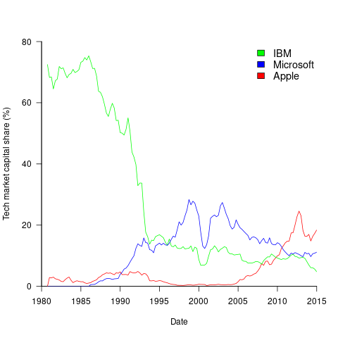
The growth of major tech companies, from the mid-1980s caused IBM’s dominant position to dramatically decline, while first Microsoft, and then Apple, grew to have more dominant market positions.
Is IBM’s decline in market valuation mirrored by a decline in its revenue?
The Fortune 500 was an annual list of the top 500 largest US companies, by total revenue (it’s now a global company list), and the lists from 1955 to 2012 are available via the Wayback Machine. Which of the 1,959 companies appearing in the top 500 lists should be classified as computer companies? Lacking a list of business classification codes for US companies, I asked Chat GPT-4 to classify these companies (responses, which include a summary of the business area). GPT-4 sometimes classified companies that were/are heavy users of computers, or suppliers of electronic components as a computer company. For instance, I consider Verizon Communications to be a communication company.
The plot below shows the ranking of those computer companies appearing within the top 100 of the Fortune 500, after removing companies not primarily in the computer business (code+data):
![]()
IBM is the uppermost blue line, ranking in the top-10 since the late-1960s. Microsoft and Apple are slowly working their way up from much lower ranks.
These contrasting plots illustrate the fact that while IBM continued to a large company by revenue, its low profitability (and major losses) and the perceived lack of a viable route to sustainable profitability resulted in it having a lower stock market valuation than computer companies with much lower revenues.
Average lines added/deleted by commits across languages
Are programs written in some programming language shorter/longer, on average, than when written in other languages?
There is a lot of variation in the length of the same program written in the same language, across different developers. Comparing program length across different languages requires a large sample of programs, each implemented in different languages, and by many different developers. This sounds like a fantasy sample, given the rarity of finding the same specification implemented multiple times in the same language.
There is a possible alternative approach to answering this question: Compare the size of commits, in lines of code, for many different programs across a variety of languages. The paper: A Study of Bug Resolution Characteristics in Popular Programming Languages by Zhang, Li, Hao, Wang, Tang, Zhang, and Harman studied 3,232,937 commits across 585 projects and 10 programming languages (between 56 and 60 projects per language, with between 58,533 and 474,497 commits per language).
The data on each commit includes: lines added, lines deleted, files changed, language, project, type of commit, lines of code in project (at some point in time). The paper investigate bug resolution characteristics, but does not include any data on number of people available to fix reported issues; I focused on all lines added/deleted. Modifying a line will be treated as an deleted/added line.
Different projects (programs) will have different characteristics. For instance, a smaller program provides more scope for adding lots of new functionality, and a larger program contains more code that can be deleted. Some projects/developers commit every change (i.e., many small commit), while others only commit when the change is completed (i.e., larger commits). There may also be algorithmic characteristics that affect the quantity of code written, e.g., availability of libraries or need for detailed bit twiddling.
It is not possible to include project-id directly in the model, because each project is written in a different language, i.e., language can be predicted from project-id. However, program size can be included as a continuous variable (only one LOC value is available, which is not ideal).
The following R code fits a basic model (the number of lines added/deleted is count data and usually small, so a Poisson distribution is assumed; given the wide range of commit sizes, quantile regression may be a better approach):
alang_mod=glm(additions ~ language+log(LOC), data=lc, family="poisson") dlang_mod=glm(deletions ~ language+log(LOC), data=lc, family="poisson") |
Some of the commits involve tens of thousands of lines (see plot below). This sounds rather extreme. So two sets of models are fitted, one with the original data and the other only including commits with additions/deletions containing less than 10,000 lines.
These models fit the mean number of lines added/deleted over all projects written in a particular language, and the models are multiplicative. As expected, the variance explained by these two factors is small, at around 5%. The two models fitted are (code+data):
 or
or  , and
, and  or
or  , where the value of
  is listed in the following table, and
  is the number of lines of code in the project:
                    Original          0 < lines < 10000
    Language     Added     Deleted     Added   Deleted
    C              1.0       1.0         1.0     1.0
    C#             1.7       1.6         1.5     1.5
    C++            1.9       2.1         1.3     1.4
    Go             1.4       1.2         1.3     1.2
    Java           0.9       1.0         1.5     1.5
    Javascript     1.1       1.1         1.3     1.6
    Objective-C    1.2       1.4         2.0     2.4
    PHP            2.5       2.6         1.7     1.9
    Python         0.7       0.7         0.8     0.8
Ruby 0.3 0.3 0.7 0.7 |
These fitted models suggest that commit addition/deletion both increase as project size increases, by around  , and that, for instance, a commit in Go adds 1.4 times as many lines as C, and delete 1.2 as many lines (averaged over all commits). Comparing adds/deletes for the same language: on average, a Go commit adds
  lines, and deletes
  lines.
There is a strong connection between the number of lines added/deleted in each commit. The plot below shows the lines added/deleted by each commit, with the red line showing a fitted regression model  (code+data):
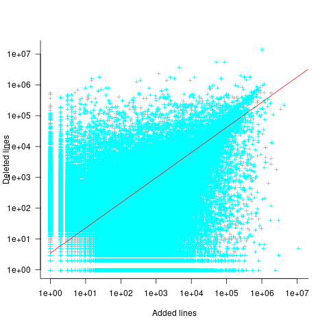
What other information can be included in a model? It is possible that project specific behavior(s) create a correlation between the size of commits; the algorithm used to fit this model assumes zero correlation. The glmer function, in the R package lme4, can take account of correlation between commits. The model component (language | project) in the following code adds project as a random effect on the language variable:
del_lmod=glmer(deletions ~ language+log(LOC)+(language | project), data=lc_loc, family=poisson) |
It takes around 24hr of cpu time to fit this model, which means I have not done much experimentation…
Software companies in the UK
How many software companies are there in the UK, and where are they concentrated?
This question begs the question of what kinds of organization should be counted as a software company. My answer to this question is driven by the available data. Companies House is the executive agency of the British Government that maintains the register of UK companies, and basic information on 5,562,234 live companies is freely available.
The Companies House data does not include all software companies. A very small company (e.g., one or two people) might decide to save on costs and paperwork by forming a partnership (companies registered at Companies House are required to file audited accounts, once a year).
When registering, companies have to specify the business domain in which they operate by selecting the appropriate Standard Industrial Classification (SIC) code, e.g., Section J: INFORMATION AND COMMUNICATION, Division 62: Computer programming, consultancy and related activities, Class 62.01: Computer programming activities, Sub-class 62.01/2: Business and domestic software development. A company’s SIC code can change over time, as the business evolves.
Searching the description associated with each SIC code, I selected the following list of SIC codes for companies likely to be considered a ‘software company’:
   62011 Ready-made interactive leisure and entertainment
                                                 software development
   62012 Business and domestic software development
   62020 Information technology consultancy activities
   62030 Computer facilities management activities
   62090 Other information technology service activities
   63110 Data processing, hosting and related activities
63120 Web portals |
There are 287,165 companies having one of these seven SIC codes (out of the 1,161 SIC codes currently used); 5.2% of all currently live companies. The breakdown is:
All 62011 62012 62020 62030 62090 63110 63120 5,562,234 7,217 68,834 134,461 3,457 57,132 7,839 8,225 100% 0.15% 1.2% 2.4% 0.06% 1.0% 0.14% 0.15% |
Only one kind of software company (SIC 62020) appears in the top ten of company SIC codes appearing in the data:
Rank SIC Companies 1 68209 232,089 Other letting and operating of own or leased real estate 2 82990 213,054 Other business support service activities n.e.c. 3 70229 211,452 Management consultancy activities other than financial management 4 68100 194,840 Buying and selling of own real estate 5 47910 165,227 Retail sale via mail order houses or via Internet 6 96090 134,992 Other service activities n.e.c. 7 62020 134,461 Information technology consultancy activities 8 99999 130,176 Dormant Company 9 98000 118,433 Residents property management 10 41100 117,264 Development of building projects |
Is the main business of a company reflected in its registered SIC code?
Perhaps a company started out mostly selling hardware with a little software, registered the appropriate non-software SIC code, but over time there was a shift to most of the income being derived from software (or the process ran in reverse). How likely is it that the SIC code will change to reflect the change of dominant income stream? I have no idea.
A feature of working as an individual contractor in the UK is that there were/are tax benefits to setting up a company, say A Ltd, and be employed by this company which invoices the company, say B Ltd, where the work is actually performed (rather than have the individual invoice B Ltd directly). IR35 is the tax legislation dealing with so-called ‘disguised’ employees (individuals who work like payroll staff, but operate and provide services via their own limited company). The effect of this practice is that what appears to be a software company in the Companies House data is actually a person attempting to be tax efficient. Unfortunately, the bulk downloadable data does not include information that might be used to filter out these cases (e.g., number of employees).
Are software companies concentrated in particular locations?
The data includes a registered address for each company. This address may be the primary business location, or its headquarters, or the location of accountants/lawyers working for the business, or a P.O. Box address. The latitude/longitude of the center of each address postcode is available. The first half of the current postcode, known as the outcode, divides the country into 2,951 areas; these outcode areas are the bins I used to count companies.
Are there areas where the probability of a company being a software company is much higher than the national average (5.265%)? The plot below shows a heat map of outcode areas having a higher than average percentage of software companies (36 out of 2,277 outcodes were at least a factor of two greater than the national average; BH7 is top with 5.9 times more companies, then RG6 with 3.7 times, BH21 with 3.6); outcodes having fewer than 10 software companies were excluded (red is highest, green lowest; code+data):
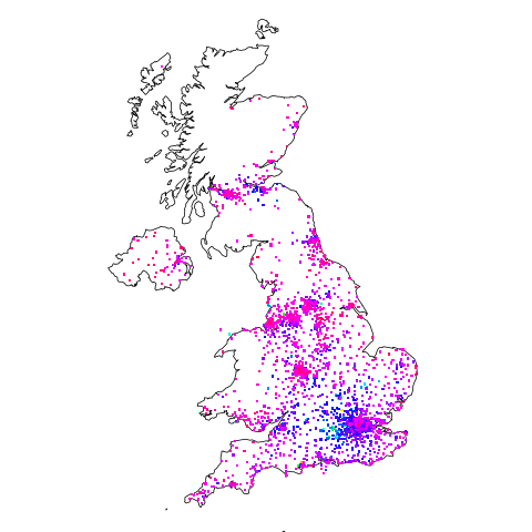
The higher concentrations are centered around the country’s traditional industrial towns and cities, with a cluster sprawling out from London. Cambridge is often cited as a high-tech region, but its highest outcode, CB4, is ranked 39th, at twice the national average (presumably the local high-tech is primarily non-software oriented).
Which outcode areas contain the most software companies? The following list shows the top ten outcodes, by number of registered companies (only BN3 and CF14 are outside London):
   Rank Outcode  Software companies
    1     WC2H      10,860
    2     EC1V       7,449
    3     N1         6,244
    4     EC2A       3,705
    5     W1W        3,205
    6     BN3        2,410
    7     CF14       2,326
    8     WC1N       2,223
    9     E14        2,192
10 SW19 1,516 |
I’m surprised to see west-central London with so many software companies. Perhaps these companies are registered at their accountants/lawyers, or they are highly paid contractors who earn enough to afford accommodation in WC2. East-central London is the location of nearly all the computer companies I know in London.
Recent Comments