Archive
Task backlog waiting times are power laws
Once it has been agreed to implement new functionality, how long do the associated tasks have to wait in the to-do queue?
An analysis of the SiP task data finds that waiting time has a power law distribution, i.e.,  , where
  is the number of tasks waiting a given amount of time; the LSST:DM Sprint/Story-point/Story has the same distribution. Is this a coincidence, or does task waiting time always have this form?
Queueing theory analyses the properties of systems involving the arrival of tasks, one or more queues, and limited implementation resources.
A basic result of queueing theory is that task waiting time has an exponential distribution, i.e., not a power law. What software task implementation behavior is sufficiently different from basic queueing theory to cause its waiting time to have a power law?
As always, my first line of attack was to find data from other domains, hopefully with an accompanying analysis modelling the behavior. It’s possible that my two samples are just way outside the norm.
Eventually I found an analysis of the letter writing response time of Darwin, Einstein and Freud (my email asking for the data has not yet received a reply). Somebody writes to a famous scientist (the scientist has to be famous enough for people to want to create a collection of their papers and letters), the scientist decides to add this letter to the pile (i.e., queue) of letters to reply to, eventually a reply is written. What is the distribution of waiting times for replies? Yes, it’s a power law, but with an exponent of -1.5, rather than -1.
The change made to the basic queueing model is to assign priorities to tasks, and then choose the task with the highest priority (rather than a random task, or the one that has been waiting the longest). Provided the queue never becomes empty (i.e., there are always waiting tasks), the waiting time is a power law with exponent -1.5; this behavior is independent of queue length and distribution of priorities (simulations confirm this behavior).
However, the exponent for my software data, and other data, is not -1.5, it is -1. A 2008 paper by Albert-László Barabási (detailed analysis) showed how a modification to the task selection process produces the desired exponent of -1. Each of the tasks currently in the queue is assigned a probability of selection, this probability is proportional to the priority of the corresponding task (i.e., the sum of the priorities/probabilities of all the tasks in the queue is assumed to be constant); task selection is weighted by this probability.
So we have a queueing model whose task waiting time is a power law with an exponent of -1. How well does this model map to software task selection behavior?
One apparent difference between the queueing model and waiting software tasks is that software tasks are assigned to a small number of priorities (e.g., Critical, Major, Minor), while each task in the model queue has a unique priority (otherwise a tie-break rule would have to be specified). In practice, I think that the developers involved do assign unique priorities to tasks.
Why wouldn’t a developer simply select what they consider to be the highest priority task to work on next?
Perhaps each developer does select what they consider to be the highest priority task, but different developers have different opinions about which task has the highest priority. The priority assigned to a task by different developers will have some probability distribution. If task priority assignment by developers is correlated, then the behavior is effectively the same as the queueing model, i.e., the probability component is supplied by different developers having different opinions and the correlation provides a clustering of priorities assigned to each task (i.e., not a uniform distribution).
If this mapping is correct, the task waiting time for a system implemented by one developer should have a power law exponent of -1.5, just like letter writing data.
The number of sprints that a story is assigned to, before being completely implemented, is a power law whose exponent varies around -3. An explanation of this behavior based on priority queues looks possible; we shall see…
The queueing models discussed above are a subset of the field known as bursty dynamics; see the review paper Bursty Human Dynamics for human behavior related aspects.
Update
A later post walking back some of the claims in this post.
Patterns in the LSST:DM Sprint/Story-point/Story ‘done’ issues
Projects that use Scrum as their project management framework estimate tasks (known as a user story, or just story) in units of Story-points. A collection of User stories are grouped together to be implemented during a Sprint (a time-boxed interval, often lasting 2-weeks).
What are Story-points, and how do they map to time (in hours and minutes)? For this post, let’s ignore these questions, simply assuming that the people who assign a story-point value to a story have some mapping in their head.
What is the average number of story-points in a story, and how does this average vary across teams? What is the distribution of number of stories estimated per sprint, how many are actually implemented, and how does this vary across teams?
The data required to answer these questions has not been publicly available, or rather public data is not known to me. Until this week, I had only known of a few public Jira repos where story-points were given for at most a few hundred stories.
The LSST Corporation, a not-for-profit involved in astronomy and physics research, has a Data Management (DM) project. The Jira repo for this project contains 26,671 ‘Done’ issues (as of Aug 2022), of which 11,082 (41.5%) have assigned story-points; there have been 469 sprints, which involved 33% of the issues. The start/end implementation date/time for stories is mostly rather granular, and not fine enough to be used to attempt to correlate individual stories with hours. I found this repo, and a couple of others, via the paper Story points changes in agile iterative development, and downloaded all available issues.
What patterns are present in the story-point and sprint data?
Story points are commonly thought of as being integer valued, but 28% of the values are non-integer. If any developers are using the Fibonacci scale, there are not enough to have a noticeable impact. The plot below shows the number of stories estimated to involve a given number of story-points (black pluses are non-integer values, which have been rounded to fit the regression model). The green curved line is a fitted biexponential (sum of two exponentials), with the two straight lines being the two component exponentials (code+data):
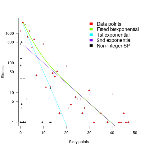
One exponential is dominant for stories assigned up to 10 story-points, and the second exponential for higher story-point values.
The development team decides to implement a story and allocates it to a sprint. A story may be reallocated to another sprint before the start of the original sprint, or after the sprint is finished when its implementation is incomplete or not yet started (the data does not allow for these cases to be distinguished). How many sprints is a story allocated to, before the story implementation is complete?
The plot below shows the number of stories allocated to a given number of sprints, with a fitted regression line of the form  (code+data):
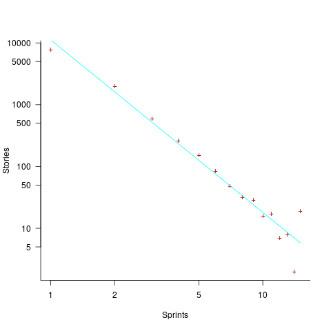
So around 14% of stories are allocated to two sprints, 5% to three and 2% to four.
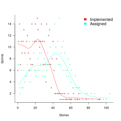
How many stories are assigned to a sprint? The plot below shows the number of sprints having a given number of stories assigned to them, and the number of sprints implementing a given number of stories; lines are fitted loess models (code+data):
Are the Story/Story-point/Sprint patterns found in the DM project likely to occur in other projects using Scrum?
I don’t know, but I hope so. Developing theories of software development processes requires that there be consistent patterns of behavior.
Not knowing what stories were assigned to a sprint at the start of the sprint, rather assigned earlier and then moved to another sprint, potentially undermines the sprint patterns. We will have to wait and see.
If anybody knows of any public Jira repos where a high percentage (say 40%) of the issues have been assigned story-points, please let me know (all the ones I know of on the Atlassian site contain a tiny percentage of story-points).
Impact of number of files on number of review comments
Code review is often discussed from the perspective of changes to a single file. In practice, code review often involves multiple files (or at least pull-based reviews do), which begs the question: Do people invest less effort reviewing files appearing later?
TLDR: The number of review comments decreases for successive files in the pull request; by around 16% per file.
The paper First Come First Served: The Impact of File Position on Code Review extracted and analysed 219,476 pull requests from 138 Java projects on Github. They also ran an experiment which asked subjects to review two files, each containing a seeded coding mistake. The paper is relatively short and omits a lot of details; I’m guessing this is due to the page limit of a conference paper.
The plot below shows the number of pull requests containing a given number of files. The colored lines indicate the total number of code review comments associated with a given pull request, with the red dots showing the 69% of pull requests that did not receive any review comments (code+data):
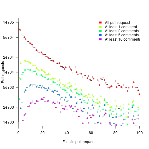
Many factors could influence the number of comments associated with a pull request; for instance, the number of people commenting, the amount of changed code, whether the code is a test case, and the number of files already reviewed (all items which happen to be present in the available data).
One factor for which information is not present in the data is social loafing, where people exert less effort when they are part of a larger group; or at least I did not find a way of easily estimating this factor.
The best model I could fit to all pull requests containing less than 10 files, and having a total of at least one comment, explained 36% of the variance present, which is not great, but something to talk about. There was a 16% decline in comments for successive files reviewed, test cases had 50% fewer comments, and there was some percentage increase with lines added; number of comments increased by a factor of 2.4 per additional commenter (is this due to importance of the file being reviewed, with importance being a metric not present in the data).
The model does not include information available in the data, such as file contents (e.g., Java, C++, configuration file, etc), and there may be correlated effects I have not taken into account. Consequently, I view the model as a rough guide.
Is the impact of file order on number of comments a side effect of some unrelated process? One way of showing a causal connection is to run an experiment.
The experiment run by the authors involved two five files, each with the first and last containing one seeded coding mistake. The 102 subjects were asked to review the two five files, with mistake file order randomly selected. The experiment looks well-structured and thought through (many are not), but the analysis of the results is confused.
The good news is that the seeded coding mistake in the first file was much more likely to be detected than the mistake in the second last file, and years of Java programming experience also had an impact (appearing first had the same impact as three years of Java experience). The bad news is that the model (a random effect model using a logistic equation) explains almost none of the variance in the data, i.e., these effects are tiny compared to whatever other factors are involved; see code+data.
What other factors might be involved?
Most experiments show a learning effect, in that subject performance improves as they perform more tasks. Having subjects review many pairs of files would enable this effect to be taken into account. Also, reviewing multiple pairs would reduce the impact of random goings-on during the review process.
The identity of the seeded mistake did not have a significant impact on the model.
Review comments are an important issue which is amenable to practical experimental investigation. I hope that the researchers run more experiments on this issue.
Analysis of a subset of the Linux Counter data
The Linux Counter project was started in 1993, with the aim of tracking the growth of Linux users (the kernel was first released two years earlier). Anybody could register any of their machines running Linux; a user ran a script that gathered basic information about a machine, and the output was emailed to the project. Once registered, users received an annual reminder to update information in their entry (despite using Linux since before the 1.0 release, user #46406 didn’t register until 2001).
When it closed (reopened/closed/coming back) it had 120K+ registered users. That’s a lot of information about computers, which unfortunately is not publicly available. I have not had any replies to my emails to those involved, asking for a copy that could be released in anonymized form.
This week I found 15,906 rows of what looks like a subset of the Linux counter data, most entries are post-2005. What did I learn from this data?
An obvious use is the pattern to check is changes over time. While the data does not include any explicit date, it does include the Kernel version, from which the earliest date can be inferred.
An earlier post used SPEC data to estimate the growth in installed memory over time; it has been doubling every 840 days, give or take. That data contains one data point per distinct vendor computer; the Linux counter data contains one entry per computer in use. There is around thirty pairs of entries for updated systems, i.e., a user updated the entry for an existing system.
The plot below shows memory installed in each registered computer, over time, for servers, laptops and workstations, with fitted regression lines. The memory size doubling times are: servers 4,000 days, laptops 2,000 days, and workstations 1,300 days (code+data):
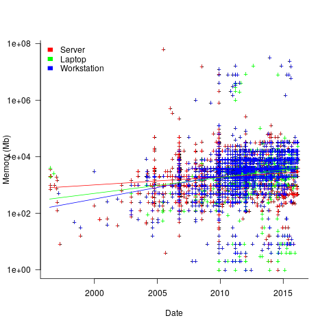
A regression model using dates is a good fit in the statistical sense, but explain very little of the variance in the data. The actual date on which the memory size was selected may have been earlier (because the kernel has been updated to a later release), or later (because memory was added, but the kernel was not updated).
Why is the memory doubling time so long?
Has memory size now reached the big-enough boundary, do Linux counter users keep the same system for many years without upgrading, are Linux counter systems retired Windows boxes that have been repurposed (data on installed memory Windows boxes would answer this point)?
Suggestions welcome.
When memory capacity is limited, it may be useful to swap least recently used memory contents to disc; Linux setup includes the specification of a swap partition. What is the optimal size of the size partition? A common recommendation is: if memory is less than 2G swap size is twice memory; if between 2-8G swap size is the same as memory, and for greater than 8G, half of memory size. The table below shows the percentage of particular system classes having a given swap/memory ratio (rounding the list of ratios to contain one decimal digit produces a list of over 100 ratio values).
swap/memory Server Workstation Laptop 1.0 15.2 19.9 25.9 2.0 10.3 9.6 8.6 0.5 9.5 7.7 8.4 |
The plot below shows memory against swap partition size, for the system classes laptop, server and workstation, with fitted regression line (code+data):
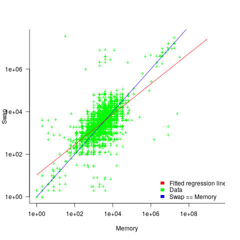
The available disk space also has a (small) impact on swap partition size; the following model explains 46% of the variance in the data:  .
.
I was hoping to confirm the rate of installed memory growth suggested by the SPEC data, with installed systems lagging a few years behind the latest releases. This Linux counter data tells a very different growth story. Perhaps pre-2005 data will tell another story (I just need to find it).
I’m not sure if the swap/memory ratio analysis is of any use to systems people. It was something of a fishing expedition on my part.
Other counting projects have included the Ubuntu counter project, and Hardware for Linux which is still active and goes back to August 2014.
I’m interested in hearing about the availability of any other Linux counter data, or data from other computer counting projects.
Recent Comments