Archive
Waiting times and the task selection process
When working on a project, what process do developers use to select the next task to implement?
One way to answer this question is to ask the developers/managers working on the project. However, these people are not always available, and sometimes the actual process used is not what management say it is.
Analysis of the amount of time a task spends in the queue finds various patterns. A previous post discussed some of the theory and data on the distribution of queue task waiting times.
What can be deduced about the task selection process from data on the time they spend in the queue?
From the theoretical perspective there are three task selection processes:
- select the task with the highest priority. The priority of a task might be set by its age (e.g., FIFO, a first, in first out queue), its value to the business, dependency of other tasks, etc.
The distribution of the number of tasks having a given waiting time on some priority queues is a power law (in a FIFO queue the waiting time distribution depends on the distribution of arrival times of new tasks), i.e.,
 , where
  is some constant
 - select a task at random. Random selection comes in various guises including: developers picking what looks to be the most interesting task on the day, or managers deciding that particular functionality would look good during a marketing/sales pitch in a few days.
The distribution of the number of tasks having a given waiting when tasks are selected at random from the queue is an exponential, i.e.,
 , where
  is some constant,
 - select a fraction,
 , of tasks by highest priority, and select the other fraction,
  , of tasks at random.
The distribution of the number of tasks having a given waiting when tasks in this process are a combination of power law and exponential, i.e.,
 , where and are constants.
The average amount of time a task spends in a queue is given by Little’s law, and is independent of the selection process (high priority tasks have a shorter waiting time than low priority tasks, but the overall average is unchanged), i.e., assuming that the averages, and variance, do not change over time, then: (waiting time) equals (average number of tasks in the queue) divided by (average number of tasks implemented per unit of time).
If analysis of the data finds just a power law, then the selection process involves a power law, just an exponential, then some random process(es), and if a combination distributions then a combination of selection processes.
Can anything be learned from knowing the value of or ?
The analysis of various priority+random models finds that, given enough running time, converges to specific values between 1 and 2. Is waiting time data on, say, 1,000 tasks (with an average of 4-hours per task, this is 2-person years) sufficient running time to converge to a good enough approximation of ?
This question can be answered by simulating task queue waiting times. The plot below shows, for 100 projects, the values of fitted to the power law component of the waiting time distribution of projects each having 1,000 tasks (the queue length was fixed at 10 tasks, five task priorities, with  fraction of tasks selected by priority, and the rest randomly; code):
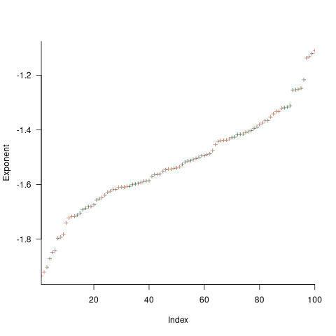
The wide range of fitted exponent values for clearly shows that 1,000 tasks is not sufficient for convergence to a good enough approximation. In fact over 100,000 tasks are needed before exponent values converge within one decimal place.
Similar results are obtained for queue lengths between 5 and 20 tasks, and priority ranges between 3 and 10. Reducing the value of down to 0.7 had a large impact on the tail of the distribution. I have not tried variable length queues.
Sometimes task priorities are changed. One study found that around 8% of bug priorities were changed before the bug was fixed. Simulation found that, when task priorities are changed (at the rate ), rather than randomly selecting a task, the waiting time distribution was a power law (also the long wait time distribution was power law like; code).
Tasks that have spent a long time in the queue are likely to have their priority increased, or be removed from the queue.
If the amount of time spent in the queue contributes some amount of priority to the original task, then the waiting time distribution is exponential (technically it is geometric, the discrete form of exponential; code). The LLM maths assistants did not find any viable equations.
To summarise: The distribution of tasks having a given waiting time has a high variance, which significantly reduces its usefulness for deducing information about the task selection process.
Example of an initial analysis of some new NASA data
For the last 20 years, the bug report databases of Open source projects have been almost the exclusive supplier of fault reports to the research community. Which, if any, of the research results are applicable to commercial projects (given the volunteer nature of most Open source projects and that anybody can submit a report)?
The only way to find out if Open source patterns are present in closed source projects is to analyse fault reports from closed source projects.
The recent paper Software Defect Discovery and Resolution Modeling incorporating Severity by Nafreen, Shi and Fiondella caught my attention for several reasons. It does non-trivial statistical analysis (most software engineering research uses simplistic techniques), it is a recent dataset (i.e., might still be available), and the data is from a NASA project (I have long assumed that NASA is more likely than most to reliable track reported issues). Lance Fiondella kindly sent me a copy of the data (paper giving more details about the data)!
Over the years, researchers have emailed me several hundred datasets. This NASA data arrived at the start of the week, and this post is an example of the kind of initial analysis I do before emailing any questions to the authors (Lance offered to answer questions, and even included two former students in his email).
It’s only worth emailing for data when there looks to be a reasonable amount (tiny samples are rarely interesting) of a kind of data that I don’t already have lots of.
This data is fault reports on software produced by NASA, a very rare sample. The 1,934 reports were created during the development and testing of software for a space mission (which launched some time before 2016).
For Open source projects, it’s long been known that many (40%) reported faults are actually requests for enhancements. Is this a consequence of allowing anybody to submit a fault report? It appears not. In this NASA dataset, 63% of the fault reports are change requests.
This data does not include any information on the amount of runtime usage of the software, so it is not possible to estimate the reliability of the software.
Software development practices vary a lot between organizations, and organizational information is often embedded in the data. Ideally, somebody familiar with the work processes that produced the data is available to answer questions, e.g., the SiP estimation dataset.
Dates form the bulk of this data, i.e., the date on which the report entered a given phase (expressed in days since a nominal start date). Experienced developers could probably guess from the column names the work performed in each phase; see list below:
    Date Created
    Date Assigned
    Date Build Integration
    Date Canceled
    Date Closed
    Date Closed With Defect
    Date In Test
    Date In Work
    Date on Hold
    Date Ready For Closure
    Date Ready For Test
    Date Test Completed
Date Work Completed |
There are probably lots of details that somebody familiar with the process would know.
What might this date information tell us? The paper cited had fitted a Cox proportional hazard model to predict fault fix time. I might try to fit a multi-state survival model.
In a priority queue, task waiting times follow a power law, while randomly selecting an item from a non-prioritized queue produces exponential waiting times. The plot below shows the number of reports taking a given amount of time (days elapsed rounded to weeks) from being assigned to build-integration, for reports at three severity levels, with fitted exponential regression lines (code+data):
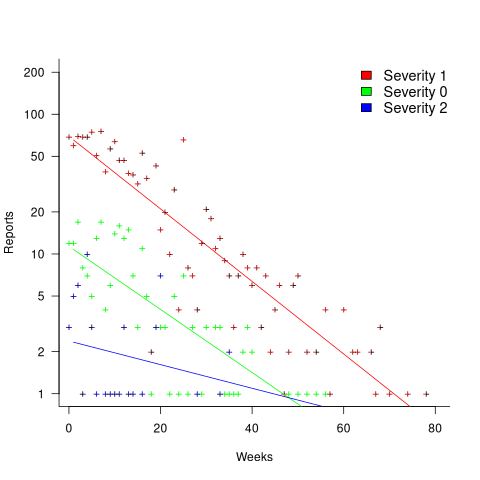
Fitting an exponential, rather than a power law, suggests that the report to handle next is effectively selected at random, i.e., reports are not in a priority queue. The number of severity 2 reports is not large enough for there to be a significant regression fit.
I now have some familiarity with the data and have spotted a pattern that may be of interest (or those involved are already aware of the random selection process).
As always, reader suggestions welcome.
Task backlog waiting times are power laws
Once it has been agreed to implement new functionality, how long do the associated tasks have to wait in the to-do queue?
An analysis of the SiP task data finds that waiting time has a power law distribution, i.e.,  , where
  is the number of tasks waiting a given amount of time; the LSST:DM Sprint/Story-point/Story has the same distribution. Is this a coincidence, or does task waiting time always have this form?
Queueing theory analyses the properties of systems involving the arrival of tasks, one or more queues, and limited implementation resources.
A basic result of queueing theory is that task waiting time has an exponential distribution, i.e., not a power law. What software task implementation behavior is sufficiently different from basic queueing theory to cause its waiting time to have a power law?
As always, my first line of attack was to find data from other domains, hopefully with an accompanying analysis modelling the behavior. It’s possible that my two samples are just way outside the norm.
Eventually I found an analysis of the letter writing response time of Darwin, Einstein and Freud (my email asking for the data has not yet received a reply). Somebody writes to a famous scientist (the scientist has to be famous enough for people to want to create a collection of their papers and letters), the scientist decides to add this letter to the pile (i.e., queue) of letters to reply to, eventually a reply is written. What is the distribution of waiting times for replies? Yes, it’s a power law, but with an exponent of -1.5, rather than -1.
The change made to the basic queueing model is to assign priorities to tasks, and then choose the task with the highest priority (rather than a random task, or the one that has been waiting the longest). Provided the queue never becomes empty (i.e., there are always waiting tasks), the waiting time is a power law with exponent -1.5; this behavior is independent of queue length and distribution of priorities (simulations confirm this behavior).
However, the exponent for my software data, and other data, is not -1.5, it is -1. A 2008 paper by Albert-László Barabási (detailed analysis) showed how a modification to the task selection process produces the desired exponent of -1. Each of the tasks currently in the queue is assigned a probability of selection, this probability is proportional to the priority of the corresponding task (i.e., the sum of the priorities/probabilities of all the tasks in the queue is assumed to be constant); task selection is weighted by this probability.
So we have a queueing model whose task waiting time is a power law with an exponent of -1. How well does this model map to software task selection behavior?
One apparent difference between the queueing model and waiting software tasks is that software tasks are assigned to a small number of priorities (e.g., Critical, Major, Minor), while each task in the model queue has a unique priority (otherwise a tie-break rule would have to be specified). In practice, I think that the developers involved do assign unique priorities to tasks.
Why wouldn’t a developer simply select what they consider to be the highest priority task to work on next?
Perhaps each developer does select what they consider to be the highest priority task, but different developers have different opinions about which task has the highest priority. The priority assigned to a task by different developers will have some probability distribution. If task priority assignment by developers is correlated, then the behavior is effectively the same as the queueing model, i.e., the probability component is supplied by different developers having different opinions and the correlation provides a clustering of priorities assigned to each task (i.e., not a uniform distribution).
If this mapping is correct, the task waiting time for a system implemented by one developer should have a power law exponent of -1.5, just like letter writing data.
The number of sprints that a story is assigned to, before being completely implemented, is a power law whose exponent varies around -3. An explanation of this behavior based on priority queues looks possible; we shall see…
The queueing models discussed above are a subset of the field known as bursty dynamics; see the review paper Bursty Human Dynamics for human behavior related aspects.
Update
A later post walking back some of the claims in this post.
Recent Comments