Archive
Waiting times and the task selection process
When working on a project, what process do developers use to select the next task to implement?
One way to answer this question is to ask the developers/managers working on the project. However, these people are not always available, and sometimes the actual process used is not what management say it is.
Analysis of the amount of time a task spends in the queue finds various patterns. A previous post discussed some of the theory and data on the distribution of queue task waiting times.
What can be deduced about the task selection process from data on the time they spend in the queue?
From the theoretical perspective there are three task selection processes:
- select the task with the highest priority. The priority of a task might be set by its age (e.g., FIFO, a first, in first out queue), its value to the business, dependency of other tasks, etc.
The distribution of the number of tasks having a given waiting time on some priority queues is a power law (in a FIFO queue the waiting time distribution depends on the distribution of arrival times of new tasks), i.e.,
 , where
  is some constant
 - select a task at random. Random selection comes in various guises including: developers picking what looks to be the most interesting task on the day, or managers deciding that particular functionality would look good during a marketing/sales pitch in a few days.
The distribution of the number of tasks having a given waiting when tasks are selected at random from the queue is an exponential, i.e.,
 , where
  is some constant,
 - select a fraction,
 , of tasks by highest priority, and select the other fraction,
  , of tasks at random.
The distribution of the number of tasks having a given waiting when tasks in this process are a combination of power law and exponential, i.e.,
 , where and are constants.
The average amount of time a task spends in a queue is given by Little’s law, and is independent of the selection process (high priority tasks have a shorter waiting time than low priority tasks, but the overall average is unchanged), i.e., assuming that the averages, and variance, do not change over time, then: (waiting time) equals (average number of tasks in the queue) divided by (average number of tasks implemented per unit of time).
If analysis of the data finds just a power law, then the selection process involves a power law, just an exponential, then some random process(es), and if a combination distributions then a combination of selection processes.
Can anything be learned from knowing the value of or ?
The analysis of various priority+random models finds that, given enough running time, converges to specific values between 1 and 2. Is waiting time data on, say, 1,000 tasks (with an average of 4-hours per task, this is 2-person years) sufficient running time to converge to a good enough approximation of ?
This question can be answered by simulating task queue waiting times. The plot below shows, for 100 projects, the values of fitted to the power law component of the waiting time distribution of projects each having 1,000 tasks (the queue length was fixed at 10 tasks, five task priorities, with  fraction of tasks selected by priority, and the rest randomly; code):
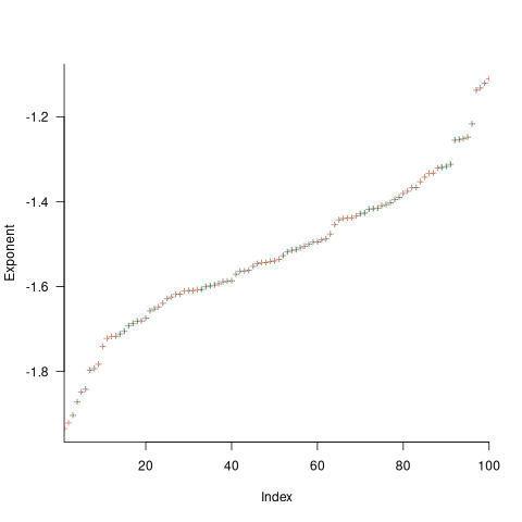
The wide range of fitted exponent values for clearly shows that 1,000 tasks is not sufficient for convergence to a good enough approximation. In fact over 100,000 tasks are needed before exponent values converge within one decimal place.
Similar results are obtained for queue lengths between 5 and 20 tasks, and priority ranges between 3 and 10. Reducing the value of down to 0.7 had a large impact on the tail of the distribution. I have not tried variable length queues.
Sometimes task priorities are changed. One study found that around 8% of bug priorities were changed before the bug was fixed. Simulation found that, when task priorities are changed (at the rate ), rather than randomly selecting a task, the waiting time distribution was a power law (also the long wait time distribution was power law like; code).
Tasks that have spent a long time in the queue are likely to have their priority increased, or be removed from the queue.
If the amount of time spent in the queue contributes some amount of priority to the original task, then the waiting time distribution is exponential (technically it is geometric, the discrete form of exponential; code). The LLM maths assistants did not find any viable equations.
To summarise: The distribution of tasks having a given waiting time has a high variance, which significantly reduces its usefulness for deducing information about the task selection process.
Projects are worked on in fits and starts
Companies whose business is designing, developing, and maintaining custom software applications (i.e., a software house) have the difficult job of keeping their expensive employees busy with paying work. Work on an existing project may be held up for various reasons, and the start date of new projects is invariably uncertain.
A solution to the on/off nature of project work is for staff to distribute their time across multiple projects. If one project is held up, there is another project available for them to book their time to.
The plot below is for project 614 in the CESAW dataset, and shows the days on which 28 people worked on this project between July 2014 and July (code+data):
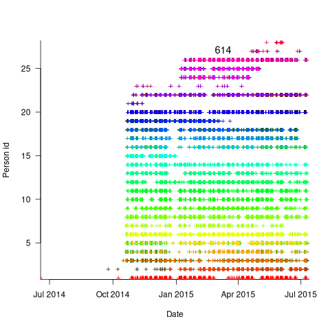
The published models of the software development lifecycle are based on perceptions of the workings of large DOD and NASA projects from the 1960s and 1970s. These projects are treated as self-contained entities, with people being available when needed and individually interchangeable. This perception fits with the software physics thinking of the time, along with the early 1960s work of Norden, and the use of differential equations to model the evolution of project manpower. These models fitted the small amount of available data as well as several other models. With some hand waving it is possible to make models such as the Putnam model look good.
With 28 people working on project 614, it’s possible that individual contributions don’t have a big impact on totals, i.e., the total time spent per week (say) does not fluctuate widely. The plot below shows the total hours per week spent on design, coding and test (total project time as roughly three staff years; code+data):
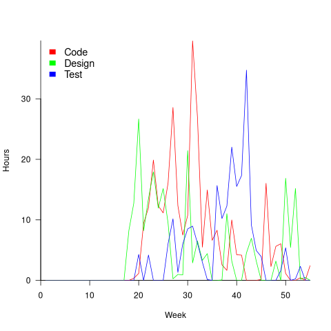
Plenty of wide fluctuations, plus some expected large drops in time spent on the project. For instance, a big drop in all activities around Christmas, and a smaller dip around Thanksgiving.
Having 28 people work on a three-person year project does seem a bit extreme (average of seven-weeks per person). On the other hand, I may be out of date, not having been a team member on a large project in decades.
The total effort required by the projects in the CESAW dataset range from three-person months to three-person years, which I suspect (no data on this question) straddles the range of time spent on the majority of software projects. The projects mostly involve people spending a non-large percentage of time on a project. The data is anonymised on a project basis, and it is not possible to count the number of projects a person is working on at any time.
To summarise: Building a good enough model of software project staffing requires taking into account organization wide staffing priorities. Existing models don’t do this.
Working with an LLM maths assistant to model software processes
This post is a overview of the techniques I use when working with LLMs as a mathematics assistant to derive equations for the aggregate behavior of a collection of software processes. Much of the following could well apply to non-software processes, but my experience is software based.
Any analysis starts with one or more questions/problems and the environment within which any answer is likely to be applicable. Possible questions include:
- Expected number of lines of code, LOC, in the next release of a program,
- number of distinct statement sequences that can be written using

if-statements and
assignmentstatements, - fraction of a program’s functions/methods that have not been modified after fixing all reported faults.
Prompting an LLM with a software related question is likely to result in it giving a software related answer summarising statements made on blogs and perhaps findings from various research papers. These summaries may, or may not, contain the desired answer.
Obtaining a mathematical answer requires that a mathematical question be asked. The software question has to be reframed in mathematical terms. This requires some creativity, lateral thinking, and prior experience is very helpful.
For instance, for question 1, expected lines of code could be reframed as a recurrence relation, such as  , where:
  is the LOC in the
  ‘th release, and
  ,
,  are constants. An LLM can solve this to relation to give an equation for based on , , and
  (the size of the first release).
A more sophisticated set of recurrence relations could include the number of developers working on the project, along the probability distribution of the number of LOC they produce per day/week/month/release, and an equation for the expected time between releases.
Expressing question 2 in mathematical terms requires some lateral thinking. One possibility is to treat each line of code as a step on a 2-D lattice. An assignment statement occupying a line is one step down the page, while an if-statement occupies both a line and is (usually) indented to the right of the previous statement at the start, and indented to the left when it ends. Paths through a lattice are a well studied problem, with lots of existing mathematics for LLMs to have been trained on. This reframing of the question was good enough for me to be able to shepherd ChatGPT towards deriving an answer to the question. My pre-LLM research for answering a related question helped.

Creating a mathematical description of a question requires a lot of hard thinking (at least it does for me), and is an iterative process. If you are lucky, a good enough mapping to a starting formula is found, and the mathematics appears in textbooks, e.g., question 1. For other questions, lateral thinking may produce a mapping to a well researched area within some mathematical niche, e.g., question 2.
Creating a correct mathematical specification of the question is essential. Get this specification wrong, and any final equation will be the answer to a different question than the one intended. Mathematicians are used to describing problems in mathematical terms, while non-mathematicians (like me, and I suspect many readers) are likely to make mistakes and under/over specify the problem.
What can be done to check whether an LLM has interpreted the question in the way intended?
LLM chain-of-thought output provides the required feedback about how it interprets the question given. Some LLMs provide chain-of-thought output of their interpretation of the information contained in the prompt (e.g., Deepseek and Kimi), while others (e.g., until recently both ChatGPT and Grok; both have improved in the last few months) provide none, i.e., they are silent for a long time before giving an answer (which is can be useful for double-checking the output from other LLMs, but is otherwise of little use).
The following discussion is based on the process I used to obtain an answer to question 3.
The number of ways of placing some number of balls in some number of boxes is an established mathematical area of study that can be mapped to question 3. Functions are treated as empty boxes and fault reports as balls that are randomly placed in these boxes.
The initial mathematical question contains the minimum of constraints, and successive questions added constraints to better mimic the characteristics of source code and fault reports.
The following was my starting question:
$m$ identical boxes can each hold a maximum of $L$ balls, and there are $b$ identical balls, balls are uniformly at randomly placed in non-full boxes, where $L < m$ and $m*L > b$ and $b$ can have a similar size as $m$ What is the expected number of boxes that do not contain a ball |
The mathematics is enclosed in $ characters. LLMs support LaTeX input and output mathematics using LaTeX.
The first two lines specify the structure of the system. It’s important to specify that the balls are identical, otherwise the LLM has to decide whether they are, or are not, identical (non-identical has a very different solution).
The third line specifies the process behavior. The phrase “uniformly at randomly” is the mathematical way of saying “the behavior is random with all possibilities being equally likely”. When I first started using LLMs, this phrase is not something I used. However, “uniformly at randomly” often appeared in LLM output, so I switched to using it (LLMs having been trained on a lot more maths than me).
Lines four and five specify relationships between variables. Sometimes constraints such as these reduce the space of possibilities, and lead to a more concise answer. These constraints specify that a function will not contain more reported faults than it has lines of code (which is not always true), and that a program will not have more reported faults than lines of code.
The last line is the question I want answered (Kimi response).
In practice functions don’t all have the same size. Most functions are short, with fewer longer ones. The number of functions containing a given number of lines has (roughly) a power law distribution. Adding this information to the problem gives:
There are $m$ boxes, $B_n$, $1 <= n <= m$ where the
number of boxes that can hold $L$ balls, $1 <= L <= T$,
is proportional to $L^{-b}$,
and there are $F$ identical balls,
balls are uniformly at randomly placed in non-full boxes,
where the number of balls $F$ is much less than
the available places to hold them.
What is the expected number of boxes that do not contain a ball |
Boxes can now have different sizes, so they need to be labelled (i.e., $B_n$), with ball carrying capacity specified as a power law, i.e., $L^{-b}$.
The explicit constraints previously given are replaced by the general statement: “… the number of balls $F$ is much less than the available places to hold them.” This gives the LLM some flexibility about how to interpret the constraint.
LLMs make mistakes. I have seen them make a basic algebra mistake on one output line, followed by output that looks like penetrating insight (if a human had made it).
The chain-of-thought output reads like a derivation that a human would write (at least it does for Kimi, Deepseek, and recently GLM 5.1 from Z.ai). Checking the correctness of this derivation is necessary to gain confidence that the final answer is correct, or not.
This chain-of-thought often makes use a theorem or identity that is new to me. Kimi’s response to the updated prompt above made use of the polylogarithm function, which I had heard of, but knew nothing about.
When new to me maths is generated, Wikipedia is the first place I look. However, some Wikipedia maths articles appear to be written by mathematicians, who assume the reader already understands the topic, and simply summarise the relevant details; which is useless. Of course, one can always ask an LLM (a different one, so there is some cross-checking).
If the chain-of-thought looks correct, is the answer correct?
An LLM once give me an answer that was obviously wrong. It was an equation that could produce negative values, and in practice only positive values were possible. Each step of the chain-of-thought looked correct. It took me a while to spot that two disjoint assumptions in the LLM analysis combined to produce the incorrect answer.
I usually have an expectation of the behavior of any answer. Plotting the value of the equation given in an answer can show whether it follows the pattern of expected behavior.
Another way of gaining confidence in the answer is to give the prompt to multiple LLMs. Sometimes they all agree, and sometimes they disagree. The disagreement may be because the answer has been written in a slightly different form (e.g., summing a series from zero rather than one), or because the LLMs made slightly different assumptions. Comparing chain-of-thought will locate the points where assumptions diverge.
The third major iteration tried to address the observation that some functions are executed more often than others, and so are more likely to be involved in a fault report.
The specification was updated to include a preferential attachment component, with a box containing a ball having a higher probability of receiving a ball than one that did not contain a ball. The added text:
balls are randomly placed in non-full boxes with probability proportional to $L*(1+O)$ where $O$ is the number of ballscurrently in the box,
The equation in the answer was rather complicated (ChatGPT response). I have not checked this equation.
Most of the mathematically oriented questions/problems I have worked on have turned out to have uninteresting answers. Knowing this I can cross them off my list of things to think about. A few might lead to something interesting (e.g., fault prediction is starting to look like a waste of time), but need more work.
The answer checking process increases confidence that a particular answer is a solution to the question asked. It is possible that the specification of the question asked does not have a strong connection to reality.
My current first choice of LLMs for mathematical problems are Deepseek, Kimi, and recently GLM 5.1 (which has compute availability issues). This is primarily because they provide chain-of-thought output. In the last few months both ChatGPT and Grok have started providing more chain-of-thought output.
I usually start with one LLM to refine the question, and depending on progress later involve other LLMs to check and verify output.
Predicting reports of new faults by counting past reports
One of the many difficulties of estimating the probability of a previously unseen fault being reported is lack of information on the amount of time spent using the application; the more time spent, the more likely a previously unseen/seen fault will be experienced. Formal prerelease testing is one of the few situations where running time is likely to be recorded.
Information that is sometimes available is the date/time of fault reports. I say sometimes because a common response to an email asking researchers for their data, is that they did not record information about duplicate faults.
What information might possibly be extracted from a time ordered list of all reported faults, i.e., including reports of previously reported faults?
My starting point for answering this questions is a previous post that analysed time to next previously unreported fault.
The following analysis treats the total number of previously reported faults as a proxy for a unit of time. The LLMs used were Deepseek (which continues to give high quality responses, which are sometimes wrong), Kimi (which is working well again, after 6–9 months of poor performance and low quality chain of thought output), ChatGPT (which now produces good quality chain of thought), Grok (which has become expressive, if not necessarily more accurate), and for the first time GLM 5.1 from the company Z.ai.
After some experimentation, the easiest to interpret formula was obtained by modelling the ‘time’ between occurrences of previously unreported faults. The following is the prompt used (this models each fault as a process that can send a signal, with the Poisson and exponential distribution requirements derived from experimental evidence; here and here):
There are $N$ independent processes. Each process, $P_i$, transmits a signal, and the number of signals transmitted in a fixed time interval, $T$, has a Poisson distribution with mean $L_i$ for $1<= i <= N$. The values $L_i$ are randomly drawn from the same exponential distribution. What is the expected number of signals transmitted by all processes between the $k$ and $k+1$ first signals from the $N$ processes. |
The LLMs responses were either (based on a weekend studying the LLM chain-of-thought response): correct (GLM), very close (ChatGPT made an assumption that was different from the one made by GLM; after some back and forth prompts between the models (via me typing them), ChatGPT agreed that GLM’s assumption was the correct one), wrong but correct when given some hints (Grok without extra help goes down a Polya urn model rabbit hole), and always wrong (Deepseek, and Kimi, which normally do very well).
The expected number of previously reported faults between the  ‘th and
 ") ‘th first occurrence of an unreported fault, is:
‘th first occurrence of an unreported fault, is:
![E[F_{prev}]={k*(2N-k-1)}/{(N-k)(N-k-1)}](https://shape-of-code.com/wp-content/plugins/wpmathpub/phpmathpublisher/img/math_977_e350e5adb969b64ebc06610cb57dd38d.png "E[F_{prev}]={k*(2N-k-1)}/{(N-k)(N-k-1)}") , where is the total number of possible distinct fault reports.
, where is the total number of possible distinct fault reports.
The variance is: (2(N-k)^2+(k-1)(N-k)+2(k-1))}/{(N-k)^2(N-k-1)^2(N-k-2)}")
While is unknown, but there is a distinctive shape to the plot of the change in the expected number of reports against (expressed as a percentage of ), as the plot below shows (see red line; code+data):
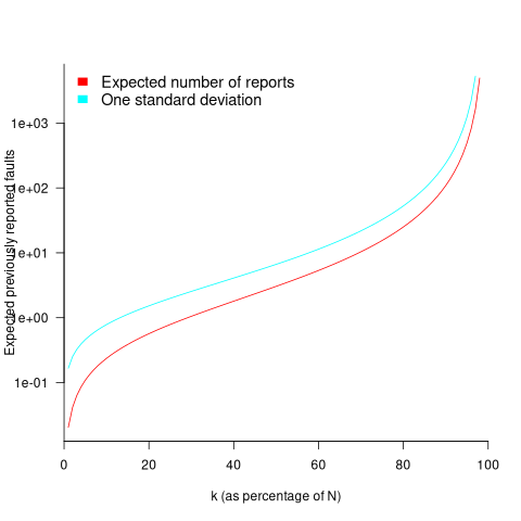
Perhaps, for a particular program, it is possible to estimate as a percentage of by comparing the relative change in the number of previously reported faults that occur between pairs of previously unreported faults.
Unfortunately the variance in the number previously reported faults completely swamps the expected value, ![E[F_{prev}]](https://shape-of-code.com/wp-content/plugins/wpmathpub/phpmathpublisher/img/math_981.5_a5ef61e64e07d16ba49517a817b2a39a.png "E[F_{prev}]") . The blue/green line in the plot above shows the upper bound of one standard deviation, with the lower bound being zero. In other words, any value between zero and the blue/green line is within one standard deviation of the expected value. There is no possibility of reliably narrowing down the bounds for , based on an estimated position of on the red curve above 🙁
. The blue/green line in the plot above shows the upper bound of one standard deviation, with the lower bound being zero. In other words, any value between zero and the blue/green line is within one standard deviation of the expected value. There is no possibility of reliably narrowing down the bounds for , based on an estimated position of on the red curve above 🙁
To quote GLM: “The variance always exceeds the mean because of two layers of randomness: the Poisson shot noise and the uncertainty in the rates themselves.”
That is the theory. Since data is available (i.e., duplicate fault reports in Apache, Eclipse and KDE), allowing the practice to be analysed (code+data).
The above analysis assumes that the software is a closed system (i.e., no code is added/modified/deleted), and that the fault report system does not attempt to reduce duplicate reports (e.g., by showing previously reported problems that appear to be similar, so the person reporting the problem may decide not to report it).
The closed system issue can be handled by analysing individual versions, but there is no solution to duplicate report reduction systems.
Across all KDE projects around 7% of reported problems were duplicates (code+data). For specific fault classes the percentage is often lower, e.g., for the konqueror project 2% of reports deal with program crashing.
Fuzzing is another source of duplicate reports. However, fuzzers are explicitly trying to exercise all parts of the code, i.e., the input is consistently different (or is intended to be).
Summary. This analysis provides another nail in the coffin of estimating the probability of encountering a previously unseen fault and of estimating the number of fault report experiences contained in a program.
Modelling time to next reported fault
After the arrival of a fault report for a program, what is the expected elapsed time until the next fault report arrives (assuming that the report relates to a coding mistake and is not a request for enhancement or something the user did wrong, and the number of active users remains the same and the program is not changed)? Here, elapsed time is a proxy for amount of program usage.
Measurements (here and here) show a consistent pattern in the elapsed time of duplicate reports of individual faults. Plotting the time elapsed between the first report and the n’th report of the same fault in the order they were reported produces an exponential line (there are often changes in the slope of this line). For example, the plot below shows 10 unique faults (different colors), the number of days between the first report and all subsequent reports of the same fault (plus character); note the log scale y-axis (discussed in this post; code+data):

The first person to report a fault may experience the same fault many times. However, they only get to submit one report. Also, some people may experience the fault and not submit a report.
If the first reporter had not submitted a report, then the time of first report would be later. Also, the time of first report could have been earlier, had somebody experienced it earlier and chosen to submit a report.
The subpopulation of users who both experience a fault and report it, decreases over time. An influx of new users is likely to cause a jump in the rate of submission of reports for previously reported faults.
It is possible to use the information on known reported faults to build a probability model for the elapsed time between the last reported known fault and the next reported known fault (time to next reported unknown fault is covered at the end of this post).
The arrival of reports for each distinct fault can be modelled as a Poisson process. The time between events in a Poisson process with rate  has an exponential distribution, with mean
  . The distribution of a sum of multiple Poisson processes is itself a Poisson process whose rate is the sum of the individual rates. The other key point is that this process is memoryless. That is, the elapsed time of any report has no impact on the elapsed time of any other report.
If there are different faults whose fitted report time exponents are:  ,
,  …
…  , then summing the Poisson rates,
  , gives the mean
  , for a probability model of the estimated time to next any-known fault report.
To summarise. Given enough duplicate reports for each fault, it’s possible to build a probability model for the time to next known fault.
In practice, people are often most interested in the time to the first report of a previous unreported fault.
tl;dr Modelling time to next previously unreported fault has an analytic solution that depends on variables whose values have to be approximately approximated.
The method used to build a probability model of reports of known fault can be used extended to build a probability model of first reports of currently unknown faults. To build this model, good enough values for the following quantities are needed:
- the number of unknown faults,
 , remaining in the program. I have some ideas about estimating the number of unknown faults, , and will discuss them in another post,
 - the time,
 , needed to have received at least one report for each of the unknown faults. In practice, this is the lifetime of the program, and there is data on software half-life. However, all coding mistakes could trigger a fault report, but not all coding mistakes will have done so during a program’s lifetime. This is a complication that needs some thought,
 - the values of
 ,
,  …
…  for each of the unknown faults. There is some data suggesting that these values are drawn from an exponential distribution, or something close to one. Also, an equation can be fitted to the values of the known faults. The analysis below assumes that the
  for each unknown fault that might be reported is randomly drawn from an exponential distribution whose mean is .
This rate will be affected by program usage (i.e., number of users and the activities they perform), and source code characteristics such as the number of executions paths that are dependent on rarely true conditions.
Putting it all together, the following is the question I asked various LLMs (which uses , rather than ):
There are independent processes. Each process,  , transmits a signal, and the number of signals transmitted in a fixed time interval, , has a Poisson distribution with mean
  for
for  . The values are randomly drawn from the same exponential distribution. What is the cumulative distribution for the time between the successive first signals from the processes.
The cumulative distribution gives the probability that an event has occurred within a given amount of time, in this case the time since the last fault report.
The ChatGPT 5.2 Thinking response (Grok Thinking gives the same formula, but no chain of thought): The probability that the  unknown fault is reported within time
  of the previous report of an unknown fault,
 ") , is given by the following rather involved formula:
, is given by the following rather involved formula:
=1-(a/{a+t})^{N-k}{}_{2}F_1(N-k, k; N+1; t/{a+t})")
where: is the initial number of faults that have not been reported,  , and
, and  is the hypergeometric function.
The important points to note are: the value  decreases as more unknown faults are reported, and the dominant contribution of the value .
Deepseek’s response also makes complicated use of the same variables, and the analysis is very similar before making some simplifications that don’t look right (text of response). Kimi’s response is usually very good, but for this question failed to handle the consequences of .
Almost all published papers on fault prediction ignore the impact of number of users on reported faults, and that report time for each distinct fault has a distinct distribution, i.e., their analysis is not connected to reality.
Best tool for measuring lots of source code
Human written source code contains various common usage patterns. This blog has analysed a variety of these patterns, and in a few cases built models of processes that replicate these patterns. The data for this analysis has primarily comes from programs written in C and Java, because these are the languages that researchers most often study (tool availability and herd mentality).
Do these common usage patterns occur in other languages, or at least other C/Java like languages? I think so, and have set out to collect the necessary data. Obtaining this data requires large quantities of code written in many languages, and the ability to analyse code written in these languages.
GitHub contains huge quantities of code. There are two freely available source code analysis tools supporting many languages: Opengrep (the Open source version of semgrep) and CodeQL.
CodeQL’s method of operation had previously put me off trying it. The method is a two stage process: First a database of information is created by extracting information during a project’s build process (e.g., running existing makefiles and host compilers), followed by querying this database using a declarative language (think minimalist SQL with lots of built-in functions). This approach has the huge advantage of not having to worry about handling compiler dialects/options, however, I’m an ingrained user of tools that process individual files.
From the research perspective, CodeQL has a major feature that is not available with other tools. GitHub, who now owns CodeQL, host thousands of project databases and GitHub Actions allows third-parties to scan up to 1,000 databases of the most popular projects. Access to existing CodeQL databases removes the need to download repo/build project/store database locally.
CodeQL, like other static analysis tools, was designed to find issues/problems in code, and so might not support the kind of functionality I needed to extract source code measurements. The best way to find out if the data of interest could be extracted is to try and do it.
In the best developer tradition, I downloaded a prebuilt release (available for Linux, Windows and Mac; called CodeQL Bundles), skimmed the documentation, ran a simple QL script and spent an hour or two trying to figure out why I was getting Java runtime errors, e.g., “no String-argument constructor/factory method to deserialize from String value“.
Progress would have been faster if I had used Visual Studio Code, available free from the owners of GitHub, rather than the command line. The documentation is not command line oriented. Visual Studio handles details like creating a qlpack.yml file (whose necessary existence I eventually found out about). Also, the harmless looking metadata appearing in comments is necessary and had better match the output parameters of the query. How hard is it to warn that a file could not be found, or that metadata is missing?
The code databases are queried using the declarative language QL, which is a kind of minimal SQL (with the select appearing last, rather than first). The import statement specifies the language, or rather the name of a library module.
The imported library contains classes for each language construct (e.g., BlockStmt, Function, ArrayExpr, etc). In the query below, the line “from LocalScopeVariable lv” extracts all local scope variables, which can subsequently be referred to via the name lv. The where line lists conditions that must be met (in this example, not be a parameter and not be accessed; testing for unused variables). The select line invokes methods that return various kinds of information about the class, e.g., the name of the variable, and location within the source.
/** * @id compound-stmt * @kind problem * @problem.severity warning */ import cpp from LocalScopeVariable lv where not lv instanceof Parameter and not exists(lv.getAnAccess()) select "", ""+lv.getName()+ ","+lv.getLocation().getStartLine()+ ","+lv.getLocation().getEndLine()+ ","+lv.getEnclosingFunction()+","+bs.getFile() |
The output generated is driven by the select, whose number/kind of arguments must match that specified by the metadata.
Developers can write and call functions, such as this one:
predicate header_suffix(string fstr) { fstr = "h" or fstr = "H" or fstr = "hpp" } |
The QL language is a declarative logical query language with roots in Datalog (subset of Prolog). The claim that it is an object-oriented language is technically correct, in that it groups functions into things called classes and supports various constructs usually found in object-oriented languages. The language has the feel of an academic project that happened to be used in a tool that was in the right place at the right time. Using host compilers to enable the tool to support many languages must have been very attractive to GitHub.
Coding in a declarative logic language requires a major mindset change. There are no loops, if statements or assignments. The query is one, potentially very long and complicated, predicate. A mindset change is necessary, but not sufficient, some fluency with the library of functions available is also needed. For instance, the isSideEffectFree predicate is true/false, but does not return a value (so there is nothing to print). I wanted to output 0/1, depending on whether a function was side effect free or not. When asked, all the LLMs questioned insisted that QL supported if-statements and assignment, just like other languages. After lots of dead-ends, an LLM claimed that “CodeQL automatically treats boolean expressions in count as 1/0″, and a test run showed this to be the case:
count(int dummy | dummy = 1 and func.isSideEffectFree() | dummy) |
The QL scripts needed to extract all the data of immediate interest to me were easily implemented. Looking at existing scripts has given me some ideas for more patterns I might measure. CodeQL currently supports 10 languages, and their classes appear to be slightly different (my initial focus is C, C++, Java and Python).
Visual Studio Code is required to run multi-repository variant analysis, i.e., scan up to 1,000 project databases on GitHub. It was after installing the CodeQL extension that I discovered how much smoother the process is within this IDE, compared to the command line (and off course the output is slightly different). There may be alternatives to Visual Studio, but I’m sticking with what the official documentation says.
Stepping back, is CodeQL a useful tool?
For me it is currently very useful, because of the large number of project databases. Some practice is needed to achieve some fluency in the use of a declarative logic language, not a major hurdle.
The need to run queries against a project database may be a major inconvenience for some developers, depending on working practices. Those practicing continuous integration should be ok.
Remotivating data analysed for another purpose
The motivation for fitting a regression model has a major impact on the model created. Some of the motivations include:
- practicing software developers/managers wanting to use information from previous work to help solve a current problem,
- researchers wanting to get their work published seeks to build a regression model that show they have discovered something worthy of publication,
- recent graduates looking to apply what they have learned to some data they have acquired,
- researchers wanting to understand the processes that produced the data, e.g., the author of this blog.
The analysis in the paper: An Empirical Study on Software Test Effort Estimation for Defense Projects by E. Cibir and T. E. Ayyildiz, provides a good example of how different motivations can produce different regression models. Note: I don’t know and have not been in contact with the authors of this paper.
I often remotivate data from a research paper. Most of the data in my Evidence-based Software Engineering book is remotivated. What a remotivation often lacks is access to the original developers/managers (this is often also true for the authors of the original paper). A complicated looking situation is often simplified by background knowledge that never got written down.
The following table shows the data appearing in the paper, which came from 15 projects implemented by a defense industry company certified at CMMI Level-3.
Proj  Test    Req   Test Meetings Faulty    Actual Scenarios
      Plan    Rev   Env          Scenarios  Effort
      Time          Time
P1    144.5  1.006    85     60     100      2850    270
P2     25.5  1.001    25.5    4       5       250     40
P3     68    1.005    42.5   32      65      1966    185
P4     85    1.002    85    104     150      3750    195
P5    198    1.007   123     87     110      3854    410
P6     57    1.006    35     25      20       903    100
P7    115    1.003    92     55      56      2143    225
P8     81    1.009   156     62      72      1988    287
P9    388    1.004   150    208     553     13246   1153
P10   177    1.008    93     77     157      4012    360
P11    62    1.001   175    186     199      5017    310
P12   111    1.005   116     82     143      3994    423
P13    63    1.009   188    177     151      3914    226
P14    32    1.008    25     28       6       435     63
P15 167 1.001 177 143 510 11555 1133 |
where: TestPlanTime is the test plan creation time in hours, ReqRev is the test/requirements review of period in hours, TestEnvTime is the test environment creation time in hours, Meetings is the number of meetings, FaultyScenarios is the number of faulty test scenarios, Scenarios is the number of Scenarios, and ActualEffort is the actual software test effort.
Industrial data is hard to obtain, so well done to the authors for obtaining this data and making it public. The authors fitted a regression model to estimate software test effort, and the model that almost perfectly fits to actual effort is:
ActualEffort=3190 + 2.65*TestPlanTime
            -3170*ReqRevPeriod - 3.5*TestEnvTime
+10.6*Meetings + 11.6*FaultScrenarios + 3.6*Scenarios |
My reading of this model is that having obtained the data, the authors felt the need to use all of it. I have been there and done that.
Why all those multiplication factors, you ask. Isn’t ActualTime simply the sum of all the work done? Yes it is, but the above table lists the work recorded, not the work done. The good news is that the fitted regression models shows that there is a very high correlation between the work done and the work recorded.
Is there a simpler model that can be used to explain/predict actual time?
Looking at the range of values in each column, ReqRev varies by just under 1%. Fitting a model that does not include this variable, we get (a slightly less perfect fit):
ActualEffort=100  + 2.0*TestPlanTime
                              - 4.3*TestEnvTime
+10.7*Meetings + 12.4*FaultScrenarios + 3.5*Scenarios |
Simple plots can often highlight patterns present in a dataset. The plot below shows every column plotted against every other column (code+data):

Points forming a straight line indicate a strong correlation, and the points in the top-right ActualEffort/FaultScrenarios plot look straight. In fact, this one variable dominates the others, and fits a model that explains over 99% of the deviation in the data:
ActualEffort=550 + 22.5*FaultScrenarios |
Many of the points in the ActualEffort/Screnarios plot are on a line, and adding Meetings data to the model explains just under 99% of the variance in the data:
actualEffort=-529.5
+15.6*Meetings + 8.7*Scenarios |
Given that FaultScrenarios is a subset of Screnarios, this connectedness is not surprising. Does the number of meetings correlate with the number of new FaultScrenarios that are discovered? Questions like this can only be answered by the original developers/managers.
The original data/analysis was interesting enough to get a paper published. Is it of interest to practicing software developers/managers?
In a small company, those involved are likely to already know what these fitted models are telling them. In a large company, the left hand does not always know what the right hand is doing. A CMMI Level-3 certified defense company is unlikely to be small, so this analysis may be of interest to some of its developer/managers.
A usable estimation model is one that only relies on information available when the estimation is needed. The above models all rely on information that only becomes available, with any accuracy, way after the estimate is needed. As such, they are not practical prediction models.
Extracting information from duplicate fault reports
Duplicate fault reports (that is, reports whose cause is the same underlying coding mistake) are an underused source of information. I sometimes email the authors of a paper analysing fault data asking for information about duplicates. Duplicate information is rarely available, because the authors don’t bother to record it.
If a program’s coding mistakes are a closed population, i.e., no new ones are added or existing ones fixed, duplicate counts might be used to estimate the number of remaining mistakes.
However, coding mistakes in production software systems are invariably open populations, i.e., reported faults are fixed, and new functionality (containing new coding mistakes) is added.
A dataset made available by Sadat, Bener, and Miranskyy contains 18 years worth of information on duplicate fault reports in Apache, Eclipse and KDE. The following analysis uses the KDE data.
Fault reports are created by users, and changes in the rate of reports whose root cause is the same coding mistake provides information on changes in the number of active users, or changes in the functionality executed by the active users. The plot below shows, for 10 unique faults (different colors), the number of days between the first report and all subsequent reports of the same fault (plus character); note the log scale y-axis (code+data):
Changes in the rate at which duplicates are reported are visible as changes in the slope of each line formed by plus signs of the respective color. Possible reasons for the change include: the coding mistake appears in a new release which users do not widely install for some time, 2) a fault become sufficiently well known, or workaround provided, that the rate of reporting for that fault declines. Of course, only some fault experiences are ever reported.
Almost all books/papers on software reliability that model the occurrence of fault experiences treat them as-if they were a Non-Homogeneous Poisson Process (NHPP); in most cases, authors are simply repeating what they have read elsewhere.
Some important assumptions made by NHPP models do not apply to software faults. For instance, NHPP models assume that the probability of encountering a fault experience is the same for different coding mistakes, i.e., they are all equally likely. What does the evidence show about this assumption? If all coding mistakes had the same probability of producing a fault experience, the mean time between duplicate fault reports would be the same for all fault reports. The plot below shows the interval, in days, between consecutive duplicate fault reports, for the 392 faults whose number of duplicates was between 20 and 100, sorted by interval (out of a total of 30,377; code+data):
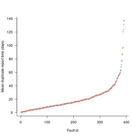
The variation in mean time between duplicate fault reports, for different faults, is evidence that different coding mistakes have different probabilities of producing a fault experience. This behavior is consistent with the observation that mistakes in deeply nested if-statements are less likely to be executed than mistakes contained in less-deeply nested code. However, this observation invalidating assumptions made by NHPP models has not prevented them dominating the research literature.
Sampling error in software engineering
In the physical sciences, measurement error occurs because of accuracy limits on the device used to make the measurement and the interpretation of the data by the person doing the measurement.
In software engineering, some measurements appear to be error free. For instance, lines of code is a discrete value that is easily counted. While some people don’t include blank lines and/or comments, the choice of what to count does not prevent an exact count being made.
In physics, the behavior of particular elements does not depend on the identity of which atoms are measured, while in software the behavior of programs written to the same specification can have different characteristics, e.g., lines of code.
For instance, each implementation of the 3n+1 problem will contain some number of LOC, with other implementations often containing a different number of LOC. The plot below shows the distribution of LOC for 6,301 implementations of 3n+1 (code and data):

Each program implementing the 3n+1 problem is one sample from the population of programs implementing the 3n+1 specification. Different people are likely to implement different programs, and the same person may create different implementations at different times.
Sampling error occurs when the characteristics of a sample are used to infer characteristics about the population from which the sample was drawn.
How might sampling error affect the results of data analysis?
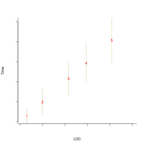
An example, using made-up values: Assume that two sets of sample measurements are made of the time taken to implement five different specifications, along with the lines of code contained in the implementations (in the same language). In the plot below, the yellow circles show a range of likely implementation measurements for each of the five specifications. The green dots, one for each specification, are measurements of one sample of programs implementing each specification; the blue dots are a second sample of programs (code):

The green and blue lines show the ordinary least squares regression model fitted to each sample. The different samples selected from the five populations has produced what appears to be slightly different models. How significant is this difference in the fitted models?
The grey line denotes where LOC is proportional to implementation time, which is one hypothesis of software project progress. The green line sample implies that LOC growth decreases as implementation time increases, while the blue line sample implies the reverse (both have been proposed as hypotheses of software project progress).
The difference in this example is important because the models fitted to the samples straddle the demarcation line between alternative theories of software project development.
A larger sample may not produce a more accurate model; a previous post analyses such a case. The example above shows a symmetric uniformly distributed population because that is the easiest to plot. In practice, populations distributions are likely to be asymmetric and irregular, e.g., measured time may be rounded to the nearest appropriate unit.
The mathematics underpinning OLS assumes that there is no error in the explanatory variables (LOC in the above plot), and that all the error is concentrated in the response variable (Time in the above plot). When there is a non-trivial sample error, or measurement error, OLS is not the appropriate technique to use to fit a regression model. The plot below shows the sample error that is assumed by OLS (code):
When there is a non-trivial error in the explanatory variable (LOC in this example), the appropriate technique for fitting a regression model is errors-in-variables regression.
Building an errors-in-variables regression model requires values for the error in the variables appearing in the equation to be fitted. Obtaining these values can be very difficult (Deming regression is a fitting technique based on the ratio of the errors).
In the above example, what is the likely variability in the implementation time and LOC, for a given specification? The limited data on the LOC contained in multiple implementations of the same specification suggests that the standard deviation of the LOC across implementations of the same specification is around 25% of the mean.
Learning researchers have run experiments where each subject performs the same task multiple times. Performance improves with practice, which makes it difficult to calculate the likely variability in the first-time performance.
My book: Evidence-based software engineering recommends using SIMEX to fit errors-in-variables models (section 11.2.3). This technique takes a model fitted using existing methods (allowing a wide range of models to be fitted), and then refits the model created based on the estimated error in one or more explanatory variables (no need to estimate an error in the response variable, the technique makes use of the value from the initial fit).
Predicting the size of the Linux kernel binary
How big is the binary for the Linux kernel? Depending on the value of around 15,000 configuration options, the size of the version 5.8 binary could be anywhere between 7.3Mb and 2,134 Mb.
Who is interested in the size of the Linux kernel binary?
We are not in the early 1980s, when memory for a desktop microcomputer often topped out at 64K, and software was distributed on 360K floppies (720K when double density arrived; my companies first product was a code optimizer which reduced program size by around 10%).
While desktop systems usually have oodles of memory (disk and RAM), developers targeting embedded systems seek to reduce costs by minimizing storage requirements, security conscious organizations want to minimise the attack surface of the programs they run, and performance critical systems might want a kernel that fits within a processors’ L2/L3 cache.
When management want to maximise the functionality supported by a kernel within given hardware resource constraints, somebody gets the job of building kernels supporting various functionality to find out the size of the binaries.
At around 4+ minutes per kernel build, it’s going to take a lot of time (or cloud costs) to compare lots of options.
The paper Transfer Learning Across Variants and Versions: The Case of Linux Kernel Size by Martin, Acher, Pereira, Lesoil, Jézéquel, and Khelladi describes an attempt to build a predictive model for the size of the kernel binary. This paper includes an extensive list of references.
The author’s approach was to first obtain lots of kernel binary sizes by building lots of kernels using random permutations of on/off options (only on/off options were changed). Seven kernel versions between 4.13 and 5.8 were used, producing 243,323 size/option setting combinations (complete dataset). This data was used to train a machine learning model.
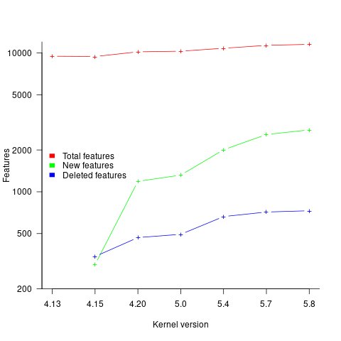
The accuracy of the predictions made by models trained on a single kernel version were accurate within that kernel version, but the accuracy of single version trained models dropped dramatically when used to predict the binary size of later kernel versions, e.g., a model trained on 4.13 had an accuracy of 5% MAPE predicting 4.13, when predicting 4.15 the accuracy is 20%, and 32% accurate predicting 5.7.
I think that the authors’ attempt to use this data to build a model that is accurate across versions is doomed to failure. The rate of change of kernel features (whose conditional compilation is supported by one or more build options) supported by Linux is too high to be accurately modelled based purely on information of past binary sizes/options. The plot below shows the total number of features, newly added, and deleted features in the modelled version of the kernel (code+data):
What is the range of impacts of each build option, on binary size?
If each build option is independent of the others (around 44% of conditional compilation directives in the kernel source contain one option), then the fitted coefficients of a simple regression model gives the build size increment when the corresponding option is enabled. After several cpu hours, the 92,562 builds involving 9,469 options in the version 4.13 build data were fitted. The plot below shows a sorted list of the size contribution of each option; the model  is 0.72, i.e., quite a good fit (code+data):
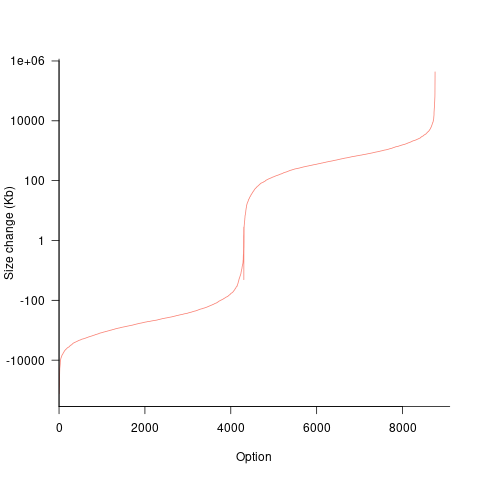
While the mean size increment for an enabled option is 75K, around 40% of enabled options decreases the size of the kernel binary. Modelling pairs of options (around 38% of conditional compilation directives in the kernel source contain two options) will have some impact on the pattern of behavior seen in the plot, but given the quality of the current model ( is 0.72) the change is unlikely to be dramatic. However, the simplistic approach of regression fitting the 90 million pairs of option interactions is not practical.
What might be a practical way of estimating binary size for any kernel version?
The size of a binary is essentially the quantity of code+static data it contains.
An estimate of the quantity of conditionally compiled source code dependent on a given option is likely to be a good proxy for that option’s incremental impact on binary size.
It’s trivial to scan source code for occurrences of options in conditional compilation directives, and with a bit more work, the number of lines controlled by the directive can be counted.
There has been a lot of evidence-based research on software product lines, and feature macros in particular. I was expecting to find a dataset listing the amount of code controlled by build options in Linux, but the data I can find does not measure Linux.
The Martin et al. build data is perfectfor creating a model linking quantity of conditionally compiled source code to change of binary size.
Recent Comments