Archive
Working with an LLM maths assistant to model software processes
This post is a overview of the techniques I use when working with LLMs as a mathematics assistant to derive equations for the aggregate behavior of a collection of software processes. Much of the following could well apply to non-software processes, but my experience is software based.
Any analysis starts with one or more questions/problems and the environment within which any answer is likely to be applicable. Possible questions include:
- Expected number of lines of code, LOC, in the next release of a program,
- number of distinct statement sequences that can be written using

if-statements and
assignmentstatements, - fraction of a program’s functions/methods that have not been modified after fixing all reported faults.
Prompting an LLM with a software related question is likely to result in it giving a software related answer summarising statements made on blogs and perhaps findings from various research papers. These summaries may, or may not, contain the desired answer.
Obtaining a mathematical answer requires that a mathematical question be asked. The software question has to be reframed in mathematical terms. This requires some creativity, lateral thinking, and prior experience is very helpful.
For instance, for question 1, expected lines of code could be reframed as a recurrence relation, such as  , where:
  is the LOC in the
  ‘th release, and
  ,
,  are constants. An LLM can solve this to relation to give an equation for based on , , and
  (the size of the first release).
A more sophisticated set of recurrence relations could include the number of developers working on the project, along the probability distribution of the number of LOC they produce per day/week/month/release, and an equation for the expected time between releases.
Expressing question 2 in mathematical terms requires some lateral thinking. One possibility is to treat each line of code as a step on a 2-D lattice. An assignment statement occupying a line is one step down the page, while an if-statement occupies both a line and is (usually) indented to the right of the previous statement at the start, and indented to the left when it ends. Paths through a lattice are a well studied problem, with lots of existing mathematics for LLMs to have been trained on. This reframing of the question was good enough for me to be able to shepherd ChatGPT towards deriving an answer to the question. My pre-LLM research for answering a related question helped.

Creating a mathematical description of a question requires a lot of hard thinking (at least it does for me), and is an iterative process. If you are lucky, a good enough mapping to a starting formula is found, and the mathematics appears in textbooks, e.g., question 1. For other questions, lateral thinking may produce a mapping to a well researched area within some mathematical niche, e.g., question 2.
Creating a correct mathematical specification of the question is essential. Get this specification wrong, and any final equation will be the answer to a different question than the one intended. Mathematicians are used to describing problems in mathematical terms, while non-mathematicians (like me, and I suspect many readers) are likely to make mistakes and under/over specify the problem.
What can be done to check whether an LLM has interpreted the question in the way intended?
LLM chain-of-thought output provides the required feedback about how it interprets the question given. Some LLMs provide chain-of-thought output of their interpretation of the information contained in the prompt (e.g., Deepseek and Kimi), while others (e.g., until recently both ChatGPT and Grok; both have improved in the last few months) provide none, i.e., they are silent for a long time before giving an answer (which is can be useful for double-checking the output from other LLMs, but is otherwise of little use).
The following discussion is based on the process I used to obtain an answer to question 3.
The number of ways of placing some number of balls in some number of boxes is an established mathematical area of study that can be mapped to question 3. Functions are treated as empty boxes and fault reports as balls that are randomly placed in these boxes.
The initial mathematical question contains the minimum of constraints, and successive questions added constraints to better mimic the characteristics of source code and fault reports.
The following was my starting question:
$m$ identical boxes can each hold a maximum of $L$ balls, and there are $b$ identical balls, balls are uniformly at randomly placed in non-full boxes, where $L < m$ and $m*L > b$ and $b$ can have a similar size as $m$ What is the expected number of boxes that do not contain a ball |
The mathematics is enclosed in $ characters. LLMs support LaTeX input and output mathematics using LaTeX.
The first two lines specify the structure of the system. It’s important to specify that the balls are identical, otherwise the LLM has to decide whether they are, or are not, identical (non-identical has a very different solution).
The third line specifies the process behavior. The phrase “uniformly at randomly” is the mathematical way of saying “the behavior is random with all possibilities being equally likely”. When I first started using LLMs, this phrase is not something I used. However, “uniformly at randomly” often appeared in LLM output, so I switched to using it (LLMs having been trained on a lot more maths than me).
Lines four and five specify relationships between variables. Sometimes constraints such as these reduce the space of possibilities, and lead to a more concise answer. These constraints specify that a function will not contain more reported faults than it has lines of code (which is not always true), and that a program will not have more reported faults than lines of code.
The last line is the question I want answered (Kimi response).
In practice functions don’t all have the same size. Most functions are short, with fewer longer ones. The number of functions containing a given number of lines has (roughly) a power law distribution. Adding this information to the problem gives:
There are $m$ boxes, $B_n$, $1 <= n <= m$ where the
number of boxes that can hold $L$ balls, $1 <= L <= T$,
is proportional to $L^{-b}$,
and there are $F$ identical balls,
balls are uniformly at randomly placed in non-full boxes,
where the number of balls $F$ is much less than
the available places to hold them.
What is the expected number of boxes that do not contain a ball |
Boxes can now have different sizes, so they need to be labelled (i.e., $B_n$), with ball carrying capacity specified as a power law, i.e., $L^{-b}$.
The explicit constraints previously given are replaced by the general statement: “… the number of balls $F$ is much less than the available places to hold them.” This gives the LLM some flexibility about how to interpret the constraint.
LLMs make mistakes. I have seen them make a basic algebra mistake on one output line, followed by output that looks like penetrating insight (if a human had made it).
The chain-of-thought output reads like a derivation that a human would write (at least it does for Kimi, Deepseek, and recently GLM 5.1 from Z.ai). Checking the correctness of this derivation is necessary to gain confidence that the final answer is correct, or not.
This chain-of-thought often makes use a theorem or identity that is new to me. Kimi’s response to the updated prompt above made use of the polylogarithm function, which I had heard of, but knew nothing about.
When new to me maths is generated, Wikipedia is the first place I look. However, some Wikipedia maths articles appear to be written by mathematicians, who assume the reader already understands the topic, and simply summarise the relevant details; which is useless. Of course, one can always ask an LLM (a different one, so there is some cross-checking).
If the chain-of-thought looks correct, is the answer correct?
An LLM once give me an answer that was obviously wrong. It was an equation that could produce negative values, and in practice only positive values were possible. Each step of the chain-of-thought looked correct. It took me a while to spot that two disjoint assumptions in the LLM analysis combined to produce the incorrect answer.
I usually have an expectation of the behavior of any answer. Plotting the value of the equation given in an answer can show whether it follows the pattern of expected behavior.
Another way of gaining confidence in the answer is to give the prompt to multiple LLMs. Sometimes they all agree, and sometimes they disagree. The disagreement may be because the answer has been written in a slightly different form (e.g., summing a series from zero rather than one), or because the LLMs made slightly different assumptions. Comparing chain-of-thought will locate the points where assumptions diverge.
The third major iteration tried to address the observation that some functions are executed more often than others, and so are more likely to be involved in a fault report.
The specification was updated to include a preferential attachment component, with a box containing a ball having a higher probability of receiving a ball than one that did not contain a ball. The added text:
balls are randomly placed in non-full boxes with probability proportional to $L*(1+O)$ where $O$ is the number of ballscurrently in the box,
The equation in the answer was rather complicated (ChatGPT response). I have not checked this equation.
Most of the mathematically oriented questions/problems I have worked on have turned out to have uninteresting answers. Knowing this I can cross them off my list of things to think about. A few might lead to something interesting (e.g., fault prediction is starting to look like a waste of time), but need more work.
The answer checking process increases confidence that a particular answer is a solution to the question asked. It is possible that the specification of the question asked does not have a strong connection to reality.
My current first choice of LLMs for mathematical problems are Deepseek, Kimi, and recently GLM 5.1 (which has compute availability issues). This is primarily because they provide chain-of-thought output. In the last few months both ChatGPT and Grok have started providing more chain-of-thought output.
I usually start with one LLM to refine the question, and depending on progress later involve other LLMs to check and verify output.
Predicting reports of new faults by counting past reports
One of the many difficulties of estimating the probability of a previously unseen fault being reported is lack of information on the amount of time spent using the application; the more time spent, the more likely a previously unseen/seen fault will be experienced. Formal prerelease testing is one of the few situations where running time is likely to be recorded.
Information that is sometimes available is the date/time of fault reports. I say sometimes because a common response to an email asking researchers for their data, is that they did not record information about duplicate faults.
What information might possibly be extracted from a time ordered list of all reported faults, i.e., including reports of previously reported faults?
My starting point for answering this questions is a previous post that analysed time to next previously unreported fault.
The following analysis treats the total number of previously reported faults as a proxy for a unit of time. The LLMs used were Deepseek (which continues to give high quality responses, which are sometimes wrong), Kimi (which is working well again, after 6–9 months of poor performance and low quality chain of thought output), ChatGPT (which now produces good quality chain of thought), Grok (which has become expressive, if not necessarily more accurate), and for the first time GLM 5.1 from the company Z.ai.
After some experimentation, the easiest to interpret formula was obtained by modelling the ‘time’ between occurrences of previously unreported faults. The following is the prompt used (this models each fault as a process that can send a signal, with the Poisson and exponential distribution requirements derived from experimental evidence; here and here):
There are $N$ independent processes. Each process, $P_i$, transmits a signal, and the number of signals transmitted in a fixed time interval, $T$, has a Poisson distribution with mean $L_i$ for $1<= i <= N$. The values $L_i$ are randomly drawn from the same exponential distribution. What is the expected number of signals transmitted by all processes between the $k$ and $k+1$ first signals from the $N$ processes. |
The LLMs responses were either (based on a weekend studying the LLM chain-of-thought response): correct (GLM), very close (ChatGPT made an assumption that was different from the one made by GLM; after some back and forth prompts between the models (via me typing them), ChatGPT agreed that GLM’s assumption was the correct one), wrong but correct when given some hints (Grok without extra help goes down a Polya urn model rabbit hole), and always wrong (Deepseek, and Kimi, which normally do very well).
The expected number of previously reported faults between the  ‘th and
 ") ‘th first occurrence of an unreported fault, is:
‘th first occurrence of an unreported fault, is:
![E[F_{prev}]={k*(2N-k-1)}/{(N-k)(N-k-1)}](https://shape-of-code.com/wp-content/plugins/wpmathpub/phpmathpublisher/img/math_977_e350e5adb969b64ebc06610cb57dd38d.png "E[F_{prev}]={k*(2N-k-1)}/{(N-k)(N-k-1)}") , where is the total number of possible distinct fault reports.
, where is the total number of possible distinct fault reports.
The variance is: (2(N-k)^2+(k-1)(N-k)+2(k-1))}/{(N-k)^2(N-k-1)^2(N-k-2)}")
While is unknown, but there is a distinctive shape to the plot of the change in the expected number of reports against (expressed as a percentage of ), as the plot below shows (see red line; code+data):
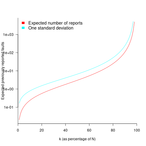
Perhaps, for a particular program, it is possible to estimate as a percentage of by comparing the relative change in the number of previously reported faults that occur between pairs of previously unreported faults.
Unfortunately the variance in the number previously reported faults completely swamps the expected value, ![E[F_{prev}]](https://shape-of-code.com/wp-content/plugins/wpmathpub/phpmathpublisher/img/math_981.5_a5ef61e64e07d16ba49517a817b2a39a.png "E[F_{prev}]") . The blue/green line in the plot above shows the upper bound of one standard deviation, with the lower bound being zero. In other words, any value between zero and the blue/green line is within one standard deviation of the expected value. There is no possibility of reliably narrowing down the bounds for , based on an estimated position of on the red curve above 🙁
. The blue/green line in the plot above shows the upper bound of one standard deviation, with the lower bound being zero. In other words, any value between zero and the blue/green line is within one standard deviation of the expected value. There is no possibility of reliably narrowing down the bounds for , based on an estimated position of on the red curve above 🙁
To quote GLM: “The variance always exceeds the mean because of two layers of randomness: the Poisson shot noise and the uncertainty in the rates themselves.”
That is the theory. Since data is available (i.e., duplicate fault reports in Apache, Eclipse and KDE), allowing the practice to be analysed (code+data).
The above analysis assumes that the software is a closed system (i.e., no code is added/modified/deleted), and that the fault report system does not attempt to reduce duplicate reports (e.g., by showing previously reported problems that appear to be similar, so the person reporting the problem may decide not to report it).
The closed system issue can be handled by analysing individual versions, but there is no solution to duplicate report reduction systems.
Across all KDE projects around 7% of reported problems were duplicates (code+data). For specific fault classes the percentage is often lower, e.g., for the konqueror project 2% of reports deal with program crashing.
Fuzzing is another source of duplicate reports. However, fuzzers are explicitly trying to exercise all parts of the code, i.e., the input is consistently different (or is intended to be).
Summary. This analysis provides another nail in the coffin of estimating the probability of encountering a previously unseen fault and of estimating the number of fault report experiences contained in a program.
Advertised prices of desktop computers during the 1990s
The 1990s was a decade of dramatic improvements in desktop computer capacity and performance. The difference in performance between the newest and current systems was clearly visible from the rate at which compiler messages zipped up the screen. How did the price of these desktop systems change during this period?
Magazine adverts are sometimes the only publicly available source of information about historical products. For instance, the characteristics of IBM PC compatible computers (e.g., price, RAM, clock frequency) over the first 20 years since they were first introduced in the early 1980s.
During the 1980s and 1990s BYTE magazine was the leading monthly computer magazine in the US, with a strong following here in the UK. Each issue contained around 400+ pages, and was packed with adverts from all the major hardware/software vendors. The last issue appeared in Jul 1998. The Internet Archive contains a scanned copy of every issue.
In 1987 Dell Computer Corp started selling cut-price computers direct to customers. Dell ran adverts in every issue of BYTE from June 1988 until the magazine closed. Gateway was another company in this market, and also regularly advertised in BYTE.
The text information present in adverts is often embedded within graphical content. My interest in this information has not been sufficient to manually type it in. LLMs are now available, and these have proven to be remarkably effective at extracting information from images.
The following advert shows how information specific to a particular computer system appears once, along with prices for particular options. Grok correctly populates a csv file containing information on four systems.
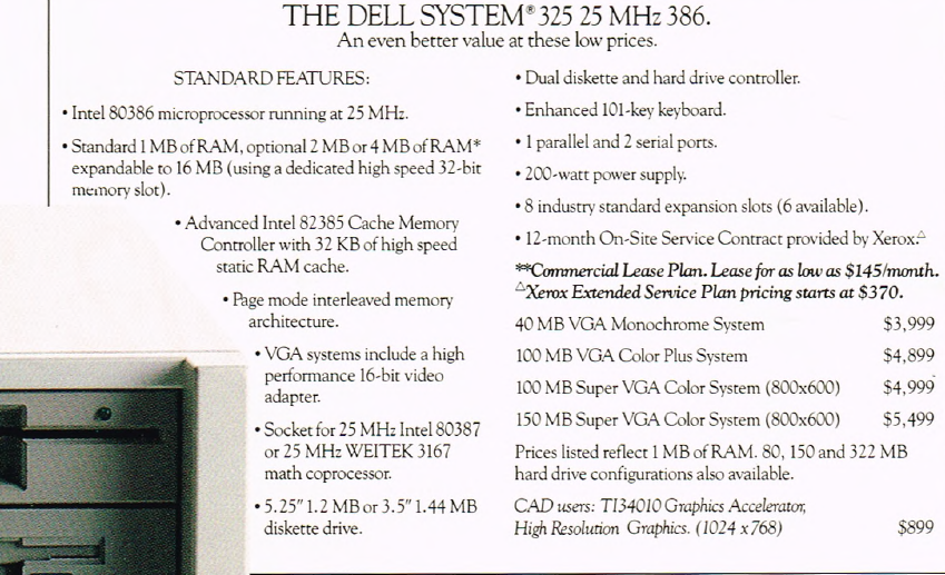
I did not attempt to ask LLMs to extract the Dell/Gateway ads from a 400+ page magazine. Manual extraction of the advert pages also gave me the opportunity to scan for other ads (a few companies advertised sporadically, e.g., Micron). Some experimentation showed that Grok returned the most accurate/reliable data.
System configuration information, for Dell and Gateway, was extracted from their adverts that appeared in the June/December issues for every year between 1988 and 1998.
Adverts show the price of particular system configurations. Typically, vendors list prices for minimal systems, along with the incremental price for more memory or a larger hard disc.
The plot below shows the original US dollar prices of 500 systems appearing in Dell/Gateway/Micron/Zeos BYTE adverts during the 1990s (code+data):
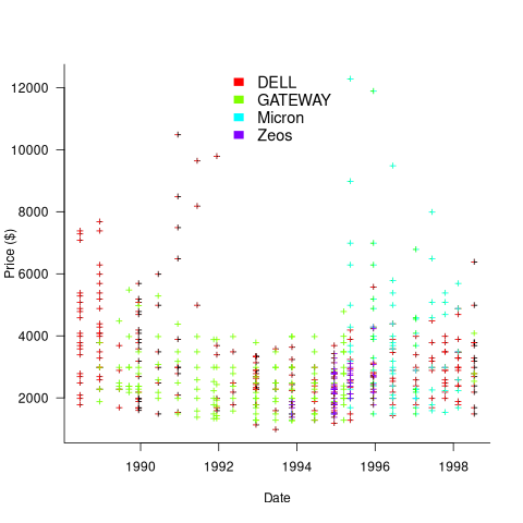
These prices have not been adjusted for inflation, and show the numeric values often ending in “99” that appeared in the adverts.
Once a ballpark figure is established in the market for the price of a product, vendors are loath to decrease it. Higher priced systems generally have higher profit margins.
Dell starts by offering systems whose price varies by a factor of four, and then settles into a narrower range of prices (presumably based on feedback from volume of sales). Micro appears to be similarly experimenting around 1996.
In the UK, when the price of low-end systems reached £1,000, rather than continuing to reduce the price, sales outlets started adding a printer to a complete package, keeping the price at around £1,000 (which families were willing to pay). Eventually the cost of a printer was not enough to fill the price gap.
The plot below shows the advertised disk size and amount of RAM installed in 500 systems advertised during the 1990s (the 1.44MB disk is a floppy drive only system; code+data):
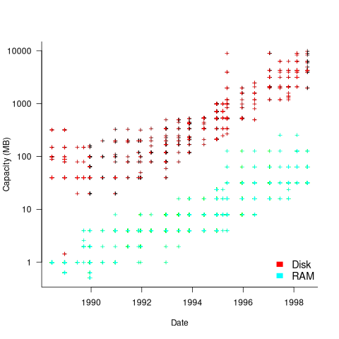
The well-known exponential capacity growth is clearly visible.
The data shows that during the 1990 there was no consistent decrease in the numeric value of the advertised price of desktop computers, which fluctuated (more data is needed to separate out the effects of functionality added to top-end systems), while actual prices decreased by 30% over the decade due to inflation. The capacity of the disk and RAM installed in desktop systems increased exponentially (also cpu clock speed; this plot is not shown).
The Hedonic index is a process used by economists to model the interaction of a product’s price and its characteristics.
Maximum Adds per second for 1950s/early 1960s computers
Relative digital computer performance has been measured, since the mid-1960s, by timing how long it takes to execute one or more programs. Until the early 1990s Whetstone was widely used, and then SPEC brought things up to date.
Running the same program on multiple computers requires that it be written in a language that is available on those computers. Fortran, Cobol and Algol 60 started to spread at the start of the 1960s (there were 21 Algol 60 compilers were available in 1961), but it took a while for old habits to change, and for specific programs to be accepted as reasonable benchmarks.
One early performance comparison method involved calculating a sum of instruction timings, weighted by instruction frequency. The view of computers as calculating machines meant that the arithmetic instructions add/multiply/divide were often the focus of attention.
A calculation based on instructions assumes that timings do not vary with the value of the operand (which multiple and divide often do, and addition sometimes does), that instruction time can be measured independent of the time taken to load the values from memory (which is not possible for when one operand is always loaded from memory), and instruction frequency is representative of typical applications.
With regard to instruction timings, some manufacturers quoted an average, while others gave a range of values. One publication quotes arithmetic timings for specific numeric values. The “Data Processing Equipment Encyclopedia: Electronic Devices”, published in 1961 by Gille Associates, lists the characteristics of 104 computers, including the time taken to perform the arithmetic operations: addition 555555+555555, multiplication 555555*555555, and division 308641358025/555555. The results were mostly for fixed point, sometimes floating-point, or both, and once in double precision. In practice small numeric values dominate program execution. I suspect the publishers picked large values because customers think of computers as working on big/complicated problems.
The time taken to load a value from memory can be a significant percentage of execution time, which is why processor cache has such a big impact on performance. In the 1950s main memory was often the cache, with the rest of memory held on a rotating drum. Hardware specifications often gave arithmetic instruction timings for both excluded and included memory access cases.
The plot below shows the execution time of the Add instruction excluding/including memory access on the same computer for pre-1961 computers, with regression line of the form:  (grey line shows
  ; code+data):
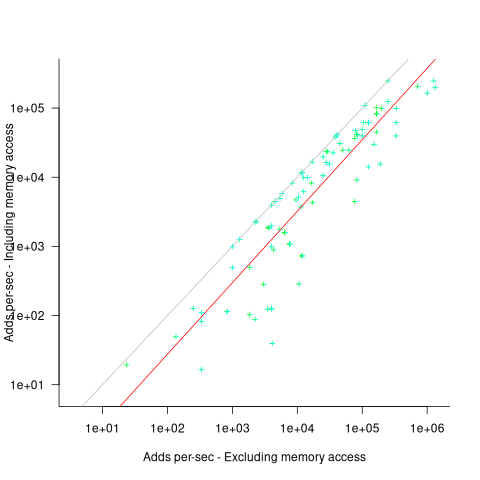
When memory access time is included in the Add instruction timing, the maximum rate of instructions per second decreases by approximately a factor of four, compared to when memory access time is excluded.
What was the frequency distribution of instructions executed by computers in the 1950s/1960s? I suspect it was a simplified form of today’s frequency distribution. Simplified in the sense of there being fewer variants of commonly used instructions and way fewer addressing modes.
Application domains were divided into scientific/engineering and commercial. One executed lots of float-point instructions, the other executed none. One did a lot of reading/writing of punched cards/magnetic tape, the other did hardly any. If we want to compare early the performance of cpus across the decades, methods that assume a significant amount of I/O have to be ignored, or the I/O component reverse engineered out.
Kenneth Knight, in his PhD thesis (no copy online), published the most detailed and extensive analysis, and data. Knight included an I/O component in his performance formula, but this was relatively small for scientific/engineering.
The table below lists the instruction weights for scientific/engineering applications published by Knight and Arbuckle, a Manager of Product Marketing at IBM:
Instruction or Operation Knight Arbuckle Floating Point Add/Sub 10% 9.5% Floating Point Multiply 6% 5.6% Floating Point Divide 2% 2.0% Fixed add/sub 10% Load/Store 28.5% Indexing 22.5% Conditional Branch 13.2% Miscellaneous 72% 18.7% |
Solomon published weights for the IBM 360 family. By focusing on a range of compatible computers the evaluation was not restricted to generic operations, and used timings from 60 different instructions.
The following analysis is based on data extracted from the 1955, 1961, and 1964 (which does not have a handy table of arithmetic instruction timings; thanks to Ed Thelen for converting the scanned images) surveys of domestic electronic digital computing systems published by the Ballistic Research Laboratory.
If the performance of computers from the 1950s/1960s is to be compared with performance in later decades, which computers from the 1950s/1960s should be included? Of the 228 computers listed in a January 1964 survey of the roughly 14k+ computing systems manufactured or operational, over 50% are bespoke, i.e., they are unique. The top 10 systems represent over 75% of manufactured systems; see table below (the IBM 604 was an electronic calculating punch, and is not listed):
   Quantity   SYSTEM           Cumulative percentage
   5,000+      IBM 1401                  36%
   2,500+      IBM 650                   54%
     693       IBM CPC                   59%
     490       LGP 30                    63%
     478       BURROUGHS B26O/B270/B280  66%
     400+      LIBRATROL 500             69%
     300+      BENDIX G-15               71%
     300       CONTROL DATA 160A         73%
     267       IBM 607                   75%
210 BURROUGHS E103/E101 77% |
When programming in machine code, developers put a lot of effort into keeping frequently used values in registers (developers can still sometimes do a better job than compilers), and overlapping memory access with other operations. The plot below shows the maximum number of add and multiply instructions per second that could be executed without accessing storage (code+data):
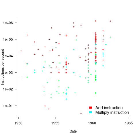
The systems capably of less than ten instructions per second are essentially early desktop calculators.
What percentage of Add instructions accessed memory? As far as I can tell, none of the performance comparison reports/papers address with this question. To be continued…
Recent Comments