Archive
Maximum Adds per second for 1950s/early 1960s computers
Relative digital computer performance has been measured, since the mid-1960s, by timing how long it takes to execute one or more programs. Until the early 1990s Whetstone was widely used, and then SPEC brought things up to date.
Running the same program on multiple computers requires that it be written in a language that is available on those computers. Fortran, Cobol and Algol 60 started to spread at the start of the 1960s (there were 21 Algol 60 compilers were available in 1961), but it took a while for old habits to change, and for specific programs to be accepted as reasonable benchmarks.
One early performance comparison method involved calculating a sum of instruction timings, weighted by instruction frequency. The view of computers as calculating machines meant that the arithmetic instructions add/multiply/divide were often the focus of attention.
A calculation based on instructions assumes that timings do not vary with the value of the operand (which multiple and divide often do, and addition sometimes does), that instruction time can be measured independent of the time taken to load the values from memory (which is not possible for when one operand is always loaded from memory), and instruction frequency is representative of typical applications.
With regard to instruction timings, some manufacturers quoted an average, while others gave a range of values. One publication quotes arithmetic timings for specific numeric values. The “Data Processing Equipment Encyclopedia: Electronic Devices”, published in 1961 by Gille Associates, lists the characteristics of 104 computers, including the time taken to perform the arithmetic operations: addition 555555+555555, multiplication 555555*555555, and division 308641358025/555555. The results were mostly for fixed point, sometimes floating-point, or both, and once in double precision. In practice small numeric values dominate program execution. I suspect the publishers picked large values because customers think of computers as working on big/complicated problems.
The time taken to load a value from memory can be a significant percentage of execution time, which is why processor cache has such a big impact on performance. In the 1950s main memory was often the cache, with the rest of memory held on a rotating drum. Hardware specifications often gave arithmetic instruction timings for both excluded and included memory access cases.
The plot below shows the execution time of the Add instruction excluding/including memory access on the same computer for pre-1961 computers, with regression line of the form:  (grey line shows
  ; code+data):
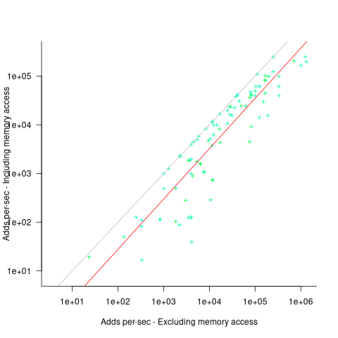
When memory access time is included in the Add instruction timing, the maximum rate of instructions per second decreases by approximately a factor of four, compared to when memory access time is excluded.
What was the frequency distribution of instructions executed by computers in the 1950s/1960s? I suspect it was a simplified form of today’s frequency distribution. Simplified in the sense of there being fewer variants of commonly used instructions and way fewer addressing modes.
Application domains were divided into scientific/engineering and commercial. One executed lots of float-point instructions, the other executed none. One did a lot of reading/writing of punched cards/magnetic tape, the other did hardly any. If we want to compare early the performance of cpus across the decades, methods that assume a significant amount of I/O have to be ignored, or the I/O component reverse engineered out.
Kenneth Knight, in his PhD thesis (no copy online), published the most detailed and extensive analysis, and data. Knight included an I/O component in his performance formula, but this was relatively small for scientific/engineering.
The table below lists the instruction weights for scientific/engineering applications published by Knight and Arbuckle, a Manager of Product Marketing at IBM:
Instruction or Operation Knight Arbuckle Floating Point Add/Sub 10% 9.5% Floating Point Multiply 6% 5.6% Floating Point Divide 2% 2.0% Fixed add/sub 10% Load/Store 28.5% Indexing 22.5% Conditional Branch 13.2% Miscellaneous 72% 18.7% |
Solomon published weights for the IBM 360 family. By focusing on a range of compatible computers the evaluation was not restricted to generic operations, and used timings from 60 different instructions.
The following analysis is based on data extracted from the 1955, 1961, and 1964 (which does not have a handy table of arithmetic instruction timings; thanks to Ed Thelen for converting the scanned images) surveys of domestic electronic digital computing systems published by the Ballistic Research Laboratory.
If the performance of computers from the 1950s/1960s is to be compared with performance in later decades, which computers from the 1950s/1960s should be included? Of the 228 computers listed in a January 1964 survey of the roughly 14k+ computing systems manufactured or operational, over 50% are bespoke, i.e., they are unique. The top 10 systems represent over 75% of manufactured systems; see table below (the IBM 604 was an electronic calculating punch, and is not listed):
   Quantity   SYSTEM           Cumulative percentage
   5,000+      IBM 1401                  36%
   2,500+      IBM 650                   54%
     693       IBM CPC                   59%
     490       LGP 30                    63%
     478       BURROUGHS B26O/B270/B280  66%
     400+      LIBRATROL 500             69%
     300+      BENDIX G-15               71%
     300       CONTROL DATA 160A         73%
     267       IBM 607                   75%
210 BURROUGHS E103/E101 77% |
When programming in machine code, developers put a lot of effort into keeping frequently used values in registers (developers can still sometimes do a better job than compilers), and overlapping memory access with other operations. The plot below shows the maximum number of add and multiply instructions per second that could be executed without accessing storage (code+data):
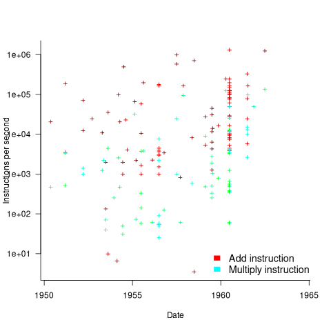
The systems capably of less than ten instructions per second are essentially early desktop calculators.
What percentage of Add instructions accessed memory? As far as I can tell, none of the performance comparison reports/papers address with this question. To be continued…
Why did organizations fund the creation of the first computers?
What were the events that drove organizations to fund the creation of the first computers?
I suspect that many readers do not appreciate how long scientific/engineering calculations took before electronic computers became available, or the huge number of clerical staff employed to process the paperwork associated with running any sizeable business.
If somebody wanted to know the logarithm of some value, or the sine/cosine of an angle, they looked up the answer in a table. Individuals owned small booklets of tables supplying some level of granularity and number of significant digits. My school boy booklet contains 60-pages of tables, all to five digits of output accuracy, with logarithm supporting four-digit input values and the sine/cosine/tangent tables having an input granularity of hundredth of a degree.
The values in these tables were calculated by human computers; with the following being among the most well known (for more details, see Calculation and Tabulation in the Nineteenth Century: Airy versus Babbage by Doron Swade, and The History of Mathematical Tables: from Sumer to Spreadsheets edited by Campbell-Kelly, Croarken, Flood, and Robson):
- In 1624 Henry Briggs published logarithms for the integer ranges 1-20,000 and 90,001-100,000 (to 14 decimal places), followed some years later by tables of sine and logarithm of sine; in 1628 Adriaan Vlacq publishing tables that filled in the missing values (to 10 decimal places). In 1783 Jurij Vega published a bug-fixed and extended version of Vlacq’s tables.
In 1827 Charles Babbage (that Babbage) published Table of Logarithms of the Natural Numbers from 1 to 10800. These tables were based on corrected versions of these tables, a rigorous nine-stage proofreading process was followed to prevent new mistakes creeping in.
Today, one person can publish A reconstruction of the tables of Briggs’ Arithmetica logarithmica (1624), with an appendix containing 300 pages of calculated values,
- between 1794 and 1799, Gaspard de Prony employed sixty to eighty computers to calculate the logarithms of the integers from 1 to 200,000 to fifteen significant digits (rounding issues sometimes required calculating 25 decimal digits; published in eighteen volumes). Around 400 man-years.
Logarithms and trigonometric functions are very widely used, creating incentives for investing in calculating and publishing tables. While it may be financially worthwhile investing in producing tables for some niche markets (e.g. Life tables for insurance companies), there is an unmet demand that will only be filled by a dramatic drop in the cost of computing simple expressions.
Babbage’s Difference engine was designed to evaluate polynomial expressions and print the results; perfect for publishing tables. While Babbage did not build a Difference engine, starting in 1837, engines based on Babbage’s design were built and sold commercially by the Swede Per Georg Scheutz.
Mechanical calculators improve accuracy and speed the process up. Vacuum tubes are invented in 1904 and become widely used to process analogue signals. World War II created an urgent demand for the results of a variety of time-consuming calculations, e.g., accurate ballistic tables, and valve computers were built. The plot below shows the cost per million operations for manual, mechanical and valve computers (code+data):
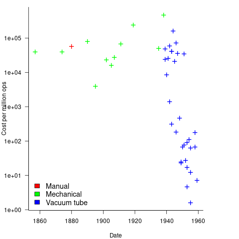
To many observers at the start of the 1950s, the market for electronic computers appeared to be organizations who needed to perform large amounts of scientific/engineering calculation.
Most businesses perform simple calculations on many unrelated values, e.g., banks have to credit/debit the appropriate account when money is deposited/withdrawn. There is no benefit in having a machine that can perform hundreds of calculations per second unless it can be fed data fast enough to keep it busy.
It so happened that, at the start of the 1950s, the US banking system was facing a crisis, the growth in the number of cheques being written meant that it would soon take longer than one day to process all the cheques that arrived in one day. In 1950 Bank of America managed 4.6 million checking accounts, and were opening 23,000 new account per month. Bank of America was then the largest bank in the world, and had a keen interest in continued growth. They funded the development of a bespoke computer system for processing cheques, the ERMA Banking system, which went live in 1959. The plot below shows the number of cheques processed per year by US banks (code+data):
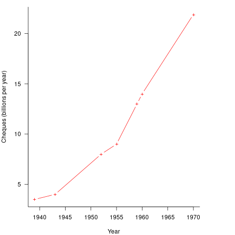
The ERMA system included electronic storage for holding account details, and data entry was speeded up by encoding account details on a magnetic strip included within every cheque.
Businesses are very interested in an integrated combination of input devices plus electronic storage plus compute. There are more commerce oriented businesses than scientific/engineering businesses, and commercial businesses usually have a lot more money to spend, i.e., the real money to be made by selling computers was the business data processing market.
The plot below shows the decreasing cost of hard disc storage (blue, right axis), along with the decreasing computing cost of valve based computers (red, left axis; code+data):
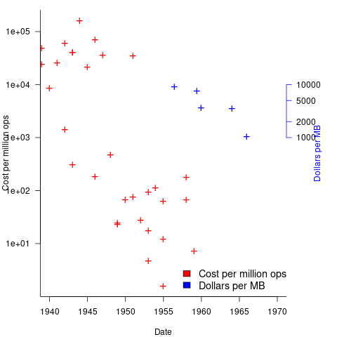
There was a larger business demand to be able to store information electronically, and the hard disc was invented by IBM, roughly 15 years after the first electronic computers.
The very different application demands of data processing and scientific/engineering are reflected in the features supported by the two languages designed in the 1950s, and widely used for the rest of the century: Cobol and Fortran.
Data processing involves simple operations on large quantities of data stored in a potentially huge number of different combinations (the myriad of mechanical point-of-sale terminals stored data in a myriad of different formats, which evolved over time, and the demand for backward compatibility created spaghetti data well before spaghetti code existed). Cobol has extensive functionality supporting the layout and format of input and output data, and simplistic coding constructs.
Scientific/engineering code involves complex calculations on some amount of input. Fortran has extensive functionality supporting program control flow, and relatively basic support for data input/output.
A third major application domain is real-time processing, such as SAGE. However, data on this domain is very hard to find, so it is not discussed.
Relative performance of computers from the 1950s/60s/70s
What was the range of performance of computers introduced in the 1950, 1960s and 1970s, and what was the annual rate of increase?
People have been measuring computer performance since they were first created, and thanks to the Internet Archive the published results are sometimes available today. The catch is that performance was often measured using different benchmarks. Fortunately, a few benchmarks were run on many systems, and in a few cases different benchmarks were run on the same system.
I have found published data on four distinct system performance estimation models, with each applied to 100+ systems (a total of 1,306 systems, of which 1,111 are unique). There is around a 20% overlap between systems across pairs of models, i.e., multiple models applied to the same system. The plot below shows the reported performance for pairs of estimates for the same system (code+data):

The relative performance relationship between pairs of different estimation models for the same system is linear (on a log scale).
Each of the models aims to produce a result that is representative of typical programs, i.e., be of use to people trying to decide which system to buy.
- Kenneth Knight built a structural model, based on 30 or so system characteristics, such as time to perform various arithmetic operations and I/O time; plugging in the values for a system produced a performance estimate. These characteristics were weighted based on measurements of scientific and commercial applications, to calculate a value that was representative of scientific or commercial operation. The Knight data appears in two magazine articles analysing systems from the 1950s and 1960s (the 310 rows are discussed in an earlier post), and the 1985 paper “A functional and structural measurement of technology”, containing data from the late 1960s and 1970s (120 rows),
- Ein-Dor and Feldmesser also built a structural model, based on the characteristics of 209 systems introduced between 1981 and 1984,
- The November 1980 Datamation article by Edward Lias lists what he called the KOPS (thousands of operations per second, i.e., MIPS for slower systems) value for 237 systems. Similar to the Knight and Ein-dor data, the calculated value is based on weighting various cpu instruction timings
- The Whetstone benchmark is based on running a particular program on a system, and recording its performance; this benchmark was designed to be representative of scientific and engineering applications, i.e., floating-point intensive. The design of this benchmark was the subject of last week’s post. I extracted 504 results from Roy Longbottom’s extensive collection of Whetstone results going back to the mid-1960s.
While the Whetstone benchmark was originally designed as an Algol 60 program that was representative of scientific applications written in Algol, only 5% of the results used this version of the benchmark; 85% of the results used the Fortran version. Fitting a regression model to the data finds that the Fortran version produced higher results than the Algol 60 version (which would encourage vendors to use the Fortran version). To ensure consistency of the Whetstone results, only those using the Fortran benchmark are used in this analysis.
A fifth dataset is the Dhrystone benchmark followed in the footsteps of the Whetstone benchmark, but targetting integer-based applications, i.e., no floating-point. First published in 1984, most of the Dhrystone results apply to more recent systems than the other benchmarks. This code+data contains the 328 results listed by the Performance Database Server.
Sometimes slightly different system names appear in the published results. I used the system names appearing in the Computers Models Database as the definitive names. It is possible that a few misspelled system names remain in the data (the possible impact is not matching systems up across models), please let me know if you spot any.
What is the best statistical technique to use to aggregate results from multiple models into a single relative performance value?
I came up with various possibilities, none of which looked that good, and even posted a question on Cross Validated (no replies yet).
Asking on the Evidence-based software engineering Discord channel produced a helpful reply from Neal Fultz, i.e., use the random effects model: lmer(log(metric) ~ (1|System)+(1|Bench), data=Sall_clean) ; after trying lots of other more complicated approaches, I would probably have eventually gotten around to using this approach.
Does this random effects model produce reliable values?
I don’t have a good idea how to evaluate the fitted model. Looking at pairs of systems where I know which is faster, the relative model values are consistent with what I know.
A csv of the calculated system relative performance values. I have yet to find a reliable way of estimating confidence bounds on these values.
The plot below shows the performance of systems introduced in a given year, on a relative scale, red line is a fitted exponential model (a factor of 5.5 faster, annually; code+data):
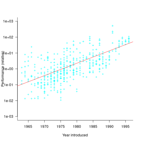
If you know of a more effective way of analysing this data, or any other published data on system benchmarks for these decades, please let me know.
Recent Comments