Relative performance of computers from the 1950s/60s/70s
What was the range of performance of computers introduced in the 1950, 1960s and 1970s, and what was the annual rate of increase?
People have been measuring computer performance since they were first created, and thanks to the Internet Archive the published results are sometimes available today. The catch is that performance was often measured using different benchmarks. Fortunately, a few benchmarks were run on many systems, and in a few cases different benchmarks were run on the same system.
I have found published data on four distinct system performance estimation models, with each applied to 100+ systems (a total of 1,306 systems, of which 1,111 are unique). There is around a 20% overlap between systems across pairs of models, i.e., multiple models applied to the same system. The plot below shows the reported performance for pairs of estimates for the same system (code+data):

The relative performance relationship between pairs of different estimation models for the same system is linear (on a log scale).
Each of the models aims to produce a result that is representative of typical programs, i.e., be of use to people trying to decide which system to buy.
- Kenneth Knight built a structural model, based on 30 or so system characteristics, such as time to perform various arithmetic operations and I/O time; plugging in the values for a system produced a performance estimate. These characteristics were weighted based on measurements of scientific and commercial applications, to calculate a value that was representative of scientific or commercial operation. The Knight data appears in two magazine articles analysing systems from the 1950s and 1960s (the 310 rows are discussed in an earlier post), and the 1985 paper “A functional and structural measurement of technology”, containing data from the late 1960s and 1970s (120 rows),
- Ein-Dor and Feldmesser also built a structural model, based on the characteristics of 209 systems introduced between 1981 and 1984,
- The November 1980 Datamation article by Edward Lias lists what he called the KOPS (thousands of operations per second, i.e., MIPS for slower systems) value for 237 systems. Similar to the Knight and Ein-dor data, the calculated value is based on weighting various cpu instruction timings
- The Whetstone benchmark is based on running a particular program on a system, and recording its performance; this benchmark was designed to be representative of scientific and engineering applications, i.e., floating-point intensive. The design of this benchmark was the subject of last week’s post. I extracted 504 results from Roy Longbottom’s extensive collection of Whetstone results going back to the mid-1960s.
While the Whetstone benchmark was originally designed as an Algol 60 program that was representative of scientific applications written in Algol, only 5% of the results used this version of the benchmark; 85% of the results used the Fortran version. Fitting a regression model to the data finds that the Fortran version produced higher results than the Algol 60 version (which would encourage vendors to use the Fortran version). To ensure consistency of the Whetstone results, only those using the Fortran benchmark are used in this analysis.
A fifth dataset is the Dhrystone benchmark followed in the footsteps of the Whetstone benchmark, but targetting integer-based applications, i.e., no floating-point. First published in 1984, most of the Dhrystone results apply to more recent systems than the other benchmarks. This code+data contains the 328 results listed by the Performance Database Server.
Sometimes slightly different system names appear in the published results. I used the system names appearing in the Computers Models Database as the definitive names. It is possible that a few misspelled system names remain in the data (the possible impact is not matching systems up across models), please let me know if you spot any.
What is the best statistical technique to use to aggregate results from multiple models into a single relative performance value?
I came up with various possibilities, none of which looked that good, and even posted a question on Cross Validated (no replies yet).
Asking on the Evidence-based software engineering Discord channel produced a helpful reply from Neal Fultz, i.e., use the random effects model: lmer(log(metric) ~ (1|System)+(1|Bench), data=Sall_clean) ; after trying lots of other more complicated approaches, I would probably have eventually gotten around to using this approach.
Does this random effects model produce reliable values?
I don’t have a good idea how to evaluate the fitted model. Looking at pairs of systems where I know which is faster, the relative model values are consistent with what I know.
A csv of the calculated system relative performance values. I have yet to find a reliable way of estimating confidence bounds on these values.
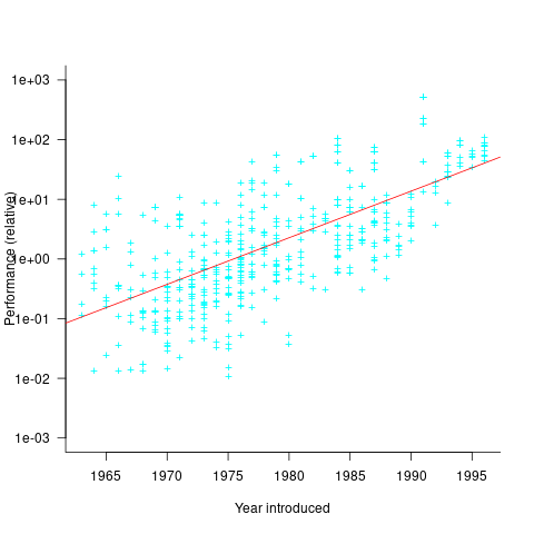
The plot below shows the performance of systems introduced in a given year, on a relative scale, red line is a fitted exponential model (a factor of 5.5 faster, annually; code+data):
If you know of a more effective way of analysing this data, or any other published data on system benchmarks for these decades, please let me know.
Here’s my arguable, flaky, but right (I tell you), view of computer performance history.
The other day, I noticed that the ratio between switching times of relay-based digital circuits and vacuum-tube based digital circuits was (very roughly) well over 1:1,000, i.e. a good, real, solid three orders of magnitude. That is, ENIAC and the like were somewhat shy of 1,000 instruction per second, but it’d be hard to perform a full-word add in anything like 1 second on a relay machine. (The Harvard/IBM Mark 1 to Mark 3 folks might disagree, of course. Still, IMHO, the tube-computer folks were held back by memory issues (core memory wasn’t until much later) and reliability issues). Bottom line: device switching speeds went from sub-audio to RF overnight.)
The next three orders of magnitude occurred between that and the KL-10 (1975) and/or* the Motorolla 68020 (1985). (As an employee of the MACSYMA group, I had access to their full KL-10 on nights, weekends, and holidays: it made a nice personal computer at the time. So I was not amused by the VAXen of that period.)
Another three orders of magnitude happenned between 1985 and 2005 or so when Intel x86 machines made it to clock speeds in the 1 to 3 GHz range, and they really could do 1 GIPS. It’s been slow since then.
*: The 10 years from the KL-10 to the 68020 were, IMHO, a matter of getting things cheaper, not faster. The idea that a Vax 11/780 was “1 MIPS” was/is, IMHO, a gross overestimate. And 68000 and 68010 workstations were terrible, but 68020 workstations were lovely; back to KL-10 levels of performance for Lisp.
@David in Tokyo
Valve computers, such as the Eniac, also had to deal with reliability issues, which meant that they were only calculating for 50-60% of the day.
I have not been able to find much data on the performance of mechanical computers. The book “Milestones in Analog and Digital Computing” contains a huge amount of data, but no timings. I emailed the author and he does not know of any.
The available data is the famous Nordhaus dataset; see figure 1 of Evidence-based software engineering.
Yes on the reliability bit. And the humongous amount of power required. (Although we’re catching with the insane wastefulness of Bitcoin and AI computing.)
The Harvard/IBM Mark 1 and later things were large enough projects that there ought to be something on their performance, I’d think.
I was reading an historical intro to computer science text, and the author bad-mouthed the valve computers something fierce, and it set me off thinking about performance, and the obvious point that relays switch in the sub- to very-low audio range whereas tubes work fine for radio/TV, so they must be 3 to 5 orders of magnitude faster instantly came to mind. (I found a current valve that han handle frequencies in the 400 GHz range, which is way faster than current transistors.)
Also, I thought the book failed to explain _why_ the ENIAC blokes went to such heroic efforts for so little comutation. We need better historians.
@David in Tokyo
Bitsavers has two interesting documents, the Manual of Operation for the Automatic Sequence Controlled Calculator has timings for basic operations and calculations (see index), and the Proceedings of a Symposium on Large-Scale Digital Calculating Machinery contains a discussion of the Bell Labs relay computers.
Given that valve elements have to be heated to around 200 C, to operate, it’s not surprising that power consumption is high. The BRL survey of digital computers has lots of details on power consumption.
I think the 400 GHz valves are essentially resonant cavities designed to produce EM waves, I’d be very surprised if they were switchable digitally.
My list of historians of computing.
Thanks for the references.