Archive
Documentation as a signal of program size
Developers and researchers invariably measure program size in lines of code, while senior managers measure by resources consumed per accounting period, e.g., money and people.
What size signals are visible to the users of a program?
Before CDs became generally available at the start of the 1990s, software for desktop computers was delivered on floppy discs that did not have the capacity to hold documentation (i.e., 128K to 1.4M), which was distributed in printed book form.
For instance, the first version of Turbo Pascal came with one 5¼ floppy (the compiler+IDE occupied 28K) and a 276-page reference manual.
Today, people are familiar with the intangible nature of software. In previous ages, people wanted to see and feel something for their money, and printed manuals were the substance they received (some products attached the floppies inside the back covers). Physical manuals were also thought to reduce software piracy (when CDs arrived, there was lots of hand-wringing over including electronic manuals).
Microsoft Windows bucked the trend, distributed with almost no physical paper, but many floppies; 13 3½ floppies for the initial upgrade to Windows 95, and 26 for Service Release 2 (oh, the fun of spending an afternoon swapping disks to rebuild a machine). Microsoft Office 97 standard edition was available on 45 floppies, the professional edition on 55.
The problem with distributing manuals in printed book form is that updates are costly; customers need a whole new book and the existing inventory needs to be scrapped. Documentation for Mainframe/Minicomputer/Workstations came in ring binders, allowing updates on an individual page basis. The Sun 4 that arrived at my office (to have a COBOL code generator written for the SPARC cpu) came with around 3-feet of ring binders. I have seen offices with a wall of shelves filled with vendor ring binders.
Is there any correlation between a project’s lines of code and pages of it’s documentation?
Most developers hate writing documentation; readmes don’t count. This means that only (well) funded development projects are likely to pay for an author to produce some amount of non-trivial documentation (a widely used application eventually attracts an external author interested in explaining things). Some Open source projects do contain files believed to be documentation; documentation research is primarily focused on accuracy (see section 6.4.4).
The only data I am aware of containing LOC, documentation page counts, and development man months is the 1979 paper The Characteristics of Large Systems by Belady and Lehman, which lists values for 37 “… independent programs developed in a large software house.” How much of the documentation was user focused, requirements+business logic, or developer focused? I have no idea (a fitted regression model, code+data, shows an almost linear relationship between LOC and document pages). Tests are not broken out as a separate item (code, documentation, not recorded?)
The plot below shows delivered: source lines of code, documentation pages, and total man months, x/y-axis both using log scales (code+data):

The total man months of implementation for each project is taken up by writing the code and documentation. The following equation is a good fit (explaining just 80% of the variance; code+data):  , but is only slightly better than
  . Given the high correlation between
  and
and  , including both in the same model is probably not a good idea (the equation:
  explains just over 50% of the variance).
There are a few possible outliers in the data. Perhaps removing these would make the picture clearer.
For me, what stands out, compared to today’s projects, is the relatively low DSLOC (a few tens of thousands) and high pages of documentation (thousands). Projects could be smaller/simpler in the 1970s because they were often replacing humans doing the work, not previously written systems; or, perhaps projects were limited by available computer memory, often well less than a megabyte. Perhaps I think the page count is high because I don’t have an accurate idea of how much online documentation is created these days.
Relative performance of computers from the 1950s/60s/70s
What was the range of performance of computers introduced in the 1950, 1960s and 1970s, and what was the annual rate of increase?
People have been measuring computer performance since they were first created, and thanks to the Internet Archive the published results are sometimes available today. The catch is that performance was often measured using different benchmarks. Fortunately, a few benchmarks were run on many systems, and in a few cases different benchmarks were run on the same system.
I have found published data on four distinct system performance estimation models, with each applied to 100+ systems (a total of 1,306 systems, of which 1,111 are unique). There is around a 20% overlap between systems across pairs of models, i.e., multiple models applied to the same system. The plot below shows the reported performance for pairs of estimates for the same system (code+data):

The relative performance relationship between pairs of different estimation models for the same system is linear (on a log scale).
Each of the models aims to produce a result that is representative of typical programs, i.e., be of use to people trying to decide which system to buy.
- Kenneth Knight built a structural model, based on 30 or so system characteristics, such as time to perform various arithmetic operations and I/O time; plugging in the values for a system produced a performance estimate. These characteristics were weighted based on measurements of scientific and commercial applications, to calculate a value that was representative of scientific or commercial operation. The Knight data appears in two magazine articles analysing systems from the 1950s and 1960s (the 310 rows are discussed in an earlier post), and the 1985 paper “A functional and structural measurement of technology”, containing data from the late 1960s and 1970s (120 rows),
- Ein-Dor and Feldmesser also built a structural model, based on the characteristics of 209 systems introduced between 1981 and 1984,
- The November 1980 Datamation article by Edward Lias lists what he called the KOPS (thousands of operations per second, i.e., MIPS for slower systems) value for 237 systems. Similar to the Knight and Ein-dor data, the calculated value is based on weighting various cpu instruction timings
- The Whetstone benchmark is based on running a particular program on a system, and recording its performance; this benchmark was designed to be representative of scientific and engineering applications, i.e., floating-point intensive. The design of this benchmark was the subject of last week’s post. I extracted 504 results from Roy Longbottom’s extensive collection of Whetstone results going back to the mid-1960s.
While the Whetstone benchmark was originally designed as an Algol 60 program that was representative of scientific applications written in Algol, only 5% of the results used this version of the benchmark; 85% of the results used the Fortran version. Fitting a regression model to the data finds that the Fortran version produced higher results than the Algol 60 version (which would encourage vendors to use the Fortran version). To ensure consistency of the Whetstone results, only those using the Fortran benchmark are used in this analysis.
A fifth dataset is the Dhrystone benchmark followed in the footsteps of the Whetstone benchmark, but targetting integer-based applications, i.e., no floating-point. First published in 1984, most of the Dhrystone results apply to more recent systems than the other benchmarks. This code+data contains the 328 results listed by the Performance Database Server.
Sometimes slightly different system names appear in the published results. I used the system names appearing in the Computers Models Database as the definitive names. It is possible that a few misspelled system names remain in the data (the possible impact is not matching systems up across models), please let me know if you spot any.
What is the best statistical technique to use to aggregate results from multiple models into a single relative performance value?
I came up with various possibilities, none of which looked that good, and even posted a question on Cross Validated (no replies yet).
Asking on the Evidence-based software engineering Discord channel produced a helpful reply from Neal Fultz, i.e., use the random effects model: lmer(log(metric) ~ (1|System)+(1|Bench), data=Sall_clean) ; after trying lots of other more complicated approaches, I would probably have eventually gotten around to using this approach.
Does this random effects model produce reliable values?
I don’t have a good idea how to evaluate the fitted model. Looking at pairs of systems where I know which is faster, the relative model values are consistent with what I know.
A csv of the calculated system relative performance values. I have yet to find a reliable way of estimating confidence bounds on these values.
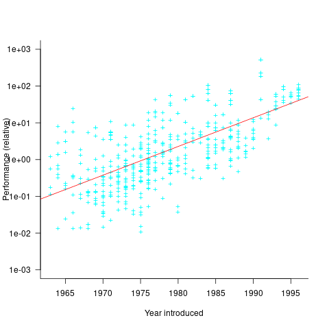
The plot below shows the performance of systems introduced in a given year, on a relative scale, red line is a fitted exponential model (a factor of 5.5 faster, annually; code+data):
If you know of a more effective way of analysing this data, or any other published data on system benchmarks for these decades, please let me know.
Recent Comments