Archive
Maximum Adds per second for 1950s/early 1960s computers
Relative digital computer performance has been measured, since the mid-1960s, by timing how long it takes to execute one or more programs. Until the early 1990s Whetstone was widely used, and then SPEC brought things up to date.
Running the same program on multiple computers requires that it be written in a language that is available on those computers. Fortran, Cobol and Algol 60 started to spread at the start of the 1960s (there were 21 Algol 60 compilers were available in 1961), but it took a while for old habits to change, and for specific programs to be accepted as reasonable benchmarks.
One early performance comparison method involved calculating a sum of instruction timings, weighted by instruction frequency. The view of computers as calculating machines meant that the arithmetic instructions add/multiply/divide were often the focus of attention.
A calculation based on instructions assumes that timings do not vary with the value of the operand (which multiple and divide often do, and addition sometimes does), that instruction time can be measured independent of the time taken to load the values from memory (which is not possible for when one operand is always loaded from memory), and instruction frequency is representative of typical applications.
With regard to instruction timings, some manufacturers quoted an average, while others gave a range of values. One publication quotes arithmetic timings for specific numeric values. The “Data Processing Equipment Encyclopedia: Electronic Devices”, published in 1961 by Gille Associates, lists the characteristics of 104 computers, including the time taken to perform the arithmetic operations: addition 555555+555555, multiplication 555555*555555, and division 308641358025/555555. The results were mostly for fixed point, sometimes floating-point, or both, and once in double precision. In practice small numeric values dominate program execution. I suspect the publishers picked large values because customers think of computers as working on big/complicated problems.
The time taken to load a value from memory can be a significant percentage of execution time, which is why processor cache has such a big impact on performance. In the 1950s main memory was often the cache, with the rest of memory held on a rotating drum. Hardware specifications often gave arithmetic instruction timings for both excluded and included memory access cases.
The plot below shows the execution time of the Add instruction excluding/including memory access on the same computer for pre-1961 computers, with regression line of the form:  (grey line shows
  ; code+data):
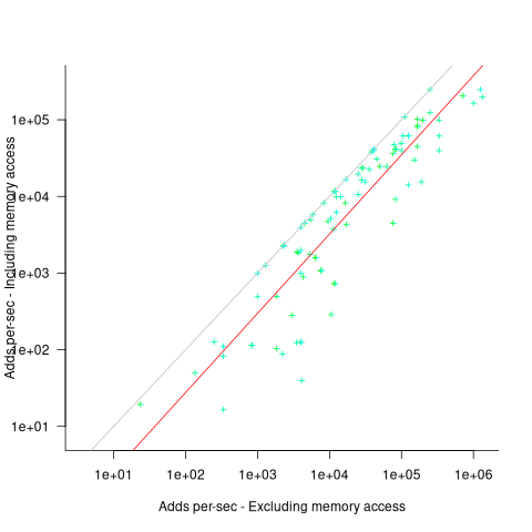
When memory access time is included in the Add instruction timing, the maximum rate of instructions per second decreases by approximately a factor of four, compared to when memory access time is excluded.
What was the frequency distribution of instructions executed by computers in the 1950s/1960s? I suspect it was a simplified form of today’s frequency distribution. Simplified in the sense of there being fewer variants of commonly used instructions and way fewer addressing modes.
Application domains were divided into scientific/engineering and commercial. One executed lots of float-point instructions, the other executed none. One did a lot of reading/writing of punched cards/magnetic tape, the other did hardly any. If we want to compare early the performance of cpus across the decades, methods that assume a significant amount of I/O have to be ignored, or the I/O component reverse engineered out.
Kenneth Knight, in his PhD thesis (no copy online), published the most detailed and extensive analysis, and data. Knight included an I/O component in his performance formula, but this was relatively small for scientific/engineering.
The table below lists the instruction weights for scientific/engineering applications published by Knight and Arbuckle, a Manager of Product Marketing at IBM:
Instruction or Operation Knight Arbuckle Floating Point Add/Sub 10% 9.5% Floating Point Multiply 6% 5.6% Floating Point Divide 2% 2.0% Fixed add/sub 10% Load/Store 28.5% Indexing 22.5% Conditional Branch 13.2% Miscellaneous 72% 18.7% |
Solomon published weights for the IBM 360 family. By focusing on a range of compatible computers the evaluation was not restricted to generic operations, and used timings from 60 different instructions.
The following analysis is based on data extracted from the 1955, 1961, and 1964 (which does not have a handy table of arithmetic instruction timings; thanks to Ed Thelen for converting the scanned images) surveys of domestic electronic digital computing systems published by the Ballistic Research Laboratory.
If the performance of computers from the 1950s/1960s is to be compared with performance in later decades, which computers from the 1950s/1960s should be included? Of the 228 computers listed in a January 1964 survey of the roughly 14k+ computing systems manufactured or operational, over 50% are bespoke, i.e., they are unique. The top 10 systems represent over 75% of manufactured systems; see table below (the IBM 604 was an electronic calculating punch, and is not listed):
   Quantity   SYSTEM           Cumulative percentage
   5,000+      IBM 1401                  36%
   2,500+      IBM 650                   54%
     693       IBM CPC                   59%
     490       LGP 30                    63%
     478       BURROUGHS B26O/B270/B280  66%
     400+      LIBRATROL 500             69%
     300+      BENDIX G-15               71%
     300       CONTROL DATA 160A         73%
     267       IBM 607                   75%
210 BURROUGHS E103/E101 77% |
When programming in machine code, developers put a lot of effort into keeping frequently used values in registers (developers can still sometimes do a better job than compilers), and overlapping memory access with other operations. The plot below shows the maximum number of add and multiply instructions per second that could be executed without accessing storage (code+data):
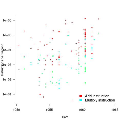
The systems capably of less than ten instructions per second are essentially early desktop calculators.
What percentage of Add instructions accessed memory? As far as I can tell, none of the performance comparison reports/papers address with this question. To be continued…
Benchmarking string search algorithms
Searching a sequence of items for occurrences of a specific pattern is a common operation, and researchers are still discovering faster string search algorithms.
While skimming the paper Efficient Exact Online String Matching Through Linked Weak Factors by M. N. Palmer, S. Faro, and S. Scafiti, Tables 1, 2 and 3 jumped out at me. The authors put a lot of effort into benchmarking the performance of 21 search algorithms representing a selection of go-faster techniques (they wanted to show that their new algorithm, using hash chains, was the fastest; Grok explains the paper). I emailed the authors for the data, and Matt Palmer kindly added it to the HashChain Github repo. Matt was also generous with his time answering my questions.
The benchmark search involved three sequences of items, each of 100MB, a genome sequence, a protein sequence and English text. The following analysis if based on results from searching the English text. The search process returned the number of occurrences of the pattern in the character sequence.
The patterns to search for were randomly extracted from the sequence being searched. Eleven pattern lengths were used, ranging from 4 to 4,096 items in powers of 2 (the tables in the paper list lengths in the range 8 to 512). There were 500 runs for each length, with a different pattern used each time, i.e., a total of 5,500 patterns. Every search algorithm matched the same 5,500 patterns.
Some algorithms have tuneable parameters (e.g., the number of characters hashed), and 107 variants of the 21 algorithms were run, giving a total of 555,067 timing measurements (a 200ms time limit sometimes prevented a run completing).
To understand some of the patterns present in the timing results, it’s necessary to know something about how industrial strength string search algorithms work. The search pattern is first processed to create either a finite state machine or some other data structure. The matching process starts at the right of the pattern and moves left, comparing items. This approach makes it possible to skip over sequences of text that cannot match. For instance, if the current text character is X, this is fed into the finite state machine created from the pattern, and if X is not in the pattern, the matching process can move forward by the length of the pattern (if the pattern contains an X, the matching process skips forward the appropriate number of characters). This pattern shift technique was first implemented in the Boyer-Moore algorithm in 1977.
One consequence of skipping over sequences that cannot match, is that longer pattern enable longer skips, resulting in faster searches. The following plot shows the search time against pattern length for two algorithms; total time includes preprocessing the pattern and searching the text (red plus symbols have been offset by 10% to show both timings; code+data):
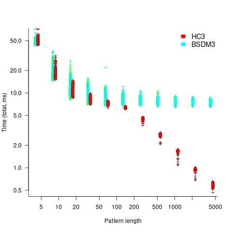
Why does the search time for HC3 (one variant of the author’s new algorithm) start to plateau and then start decreasing again? One possible cause of this saddle point is the cpu cache line width, which is 64 bytes on the system that ran the benchmarks. When the skip length is at least twice the cache line width, it is not necessary to read characters that would cause the filling of at least one cache line. As always, further research is needed.
What is the most informative method for comparing the algorithm/tool performance?
The most commonly used method is to compare mean performance times, and this is what the authors do for each pattern length. A related alternative, given that different patterns are used for each run, is to compare median times, on the basis that users are interested in the fastest algorithm across many patterns. When variance in the search times is taken into account, there is no clear winner across all pattern lengths (the uncertainty in the mean value is sometimes larger than the difference in performance).
Comparing performance across pattern lengths is interesting for algorithm designers, but users want a single performance value. The traditional approach to building a single model, that would include pattern length and algorithm, is to fit a regression model. However, this approach requires that the change in performance with pattern length roughly have the same form across all algorithms. The plot above clearly shows two algorithms with different forms of change of timing behavior with pattern length (other algorithms exhibit different behaviors).
A completely different modelling approach is to treat each pattern search as a competition between algorithms, with algorithms ranked by search time (fastest first). In this approach, the relative performance of each algorithm is ranked; there are 500 ranks for each pattern length. The fitted model can be used to calculate the probability, over all patterns, that algorithm A1 will be faster than algorithm A2.
Readers might be familiar with the Bradley-Terry model, where two items are ranked, e.g., the results from football games played between pairs of teams during a season. When more than two items are ranked, a Plackett-Luce model can be fitted. The output from fitting these models is a value,  , for each of the algorithms, e.g.,
  . The probability that algorithm
 A1 will rank higher than Algorithm A2 is calculated from the expression:
 , this expression can also be written as:
Switch A1 and A2 to calculate the opposite ranking.
The probability that algorithm A1 ranks higher than Algorithm A2 which in turn ranks higher than Algorithm A3 is calculated as follows (and so on for more algorithms):

For ease of comparison, only the 53 algorithms with 500 sets of timing data for all pattern lengths was fitted. The following plot shows the fitted values for each algorithm (blue/green lines are standard errors, and names containing HC are some variant of the authors’ hash chain technique; code+data):
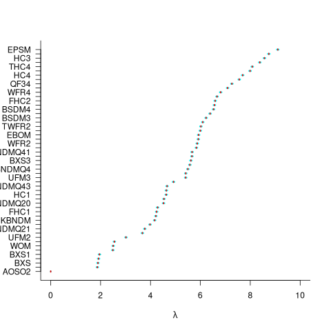
The EPSM algorithm makes use of the SSE and AVX instructions, supported by modern x86 processors, that can operate on up to 512 bits at a time.
The following table lists the fitted lambda values for the top eight ranked algorithm implementation:
 Algorithm    Lambda
      EPSM    9.103007
      THC3    8.743377
       HC3    8.567715
      FHC3    8.381220
      THC4    8.079716
      FHC4    7.991929
       HC4    7.695787
TWFR4 7.557796 |
The likelihood that EPSM will rank higher than THC3 is } right 0.59") .
.
This is better than random, and reflects the variability in algorithm performance, i.e., there is no clear winner.
It might be possible to extract more information from the data.
Some algorithms use of the same technique for part of their search process. Information on the techniques shared by algorithms can be added to the model as covariates. Assuming that a suitable fit is obtained, the model coefficients would indicate the relative impact of each technique on performance. I don’t know enough to select the techniques, and Matt is thinking about it.
CPU frequency not relevant to SPEC benchmark performance
Despite the end of Dennard scaling around 2005-7 computer performance, as measured by the SPEC cpu benchmarks, continues to improve. What is driving this ongoing increase in performance, given that cpu clock rates have stopped increasing?
The plot below shows 9,161 results from the SPEC CPU integer benchmark, plus the fitted regression line  (code+data):
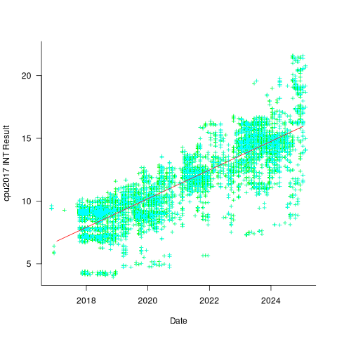
There is a scattering of benchmark results because manufacturers offer systems having a range of performance.
Possible factors driving the ongoing increases in system performance include increased DRAM-memory bandwidth, and cpu improvements such as larger caches and more accurate branch prediction. While Moore’s law (i.e., rate of growth of the number of transistors on a chip) has slowed down a lot, the number of transistors in a processor chip has continued to increase (many of these transistors have been used to build chips that contain multiple cpu cores).
The SPEC benchmark result data includes a lot of information about the system that ran the benchmarks, including: processor family/model, number of cpu cores, clock frequency, amount of memory installed and its type.
Results from SPEC CPU2017, the current version of the benchmark, are available from the start of 2017 to now. The following analysis uses these results. Results from the SPEC CPU2006 benchmark are also available, and a regression model fitted to the results from the 780 systems that ran both benchmarks, gives the mapping from CPU INT 2006 to CPU INT 2017 as:  .
.
The processor information in the results file usually specifies family name plus model number/name. The model information usually correlates with clock frequency, perhaps cache size, or gpu support; some examples below.
    AMD EPYC 4464P                AMD EPYC 4564P
    AMD Ryzen 9 7950X             AMD Ryzen 7 5800X
    Intel Xeon Platinum 8490H     Intel Xeon Gold 6438N
Intel Xeon E3-1220 v3 Intel Xeon E5-2697 v3 |
The family name is sufficient for an initial analysis. Details of any cache size differences between models can always be included in a later analysis. The following table shows the number of processor x86 based families present in the 2017 INT results (total 9,161):
           AMD EPYC           AMD Ryzen               Intel
               1475                   7                   1
      Intel Celeron       Intel Core i3       Intel Core i5
                 16                  31                   2
      Intel Core i7       Intel Pentium          Intel Xeon
                  1                  30                 605
  Intel Xeon Bronze        Intel Xeon D       Intel Xeon E3
                167                  12                  16
      Intel Xeon E5       Intel Xeon E7     Intel Xeon Gold
                  3                   2                3994
Intel Xeon Platinum   Intel Xeon Silver        Intel Xeon W
1822 969 8 |
The memory information usually includes total bytes, number of memory sticks and interface standard (e.g., DDR2/3/4/5); some examples below.
    64 GB (2 x 32 GB 2Rx4 PC5-5600B-R, running at 5200)
    64 GB (2 x 32 GB 2Rx8 PC4-3200AA-E)
    256 GB (8*1GB DDR2-400 DIMMS per 4 core module)
    192 GB (4 x 12 x 4 GB DDR3-1333R, ECC, CL9)
    32 GB (8 x 4 GB Dual-rank PC2-6400 CL5-5-5 FB-DIMMs)
24 GB (6 x 4 GB DDR3-1333 downclocked to 1066 MHz) |
The memory bandwidth can be calculated from the interface standard used. The names of modern DRAM interface standards start with either DDR or PC, and a number, a hyphen and then another number. The values appearing in the SPEC results don’t always follow the naming rules listed in the standard (e.g., last number of a PC name using the corresponding DDR number), and in a few cases a digit was dropped from the last number. Where possible the ‘obvious’ edits were made (sometimes values were just wrong), see code for details. The following table shows the number of interface standards represented in the 2017 CPU INT results (total 9,161; in the 2006 results DDR names predominated):
PC4-2400  PC4-2666  PC4-2933  PC4-3200  PC4-4800 PC5-11200 PC5-12800
      26      2248      2163      2080         6         2         3
PC5-4800  PC5-5200  PC5-5600  PC5-6400     PC5-8  PC5-8800
1735 5 653 233 2 5 |
Once the memory is identified, its bandwidth can be looked up (bespoke memory stick clock rates were ignored). Fitting a regression model to the data, with the CPU INT (cpu integer benchmark) result as the outcome, we get (using a multiplicative model allows each factor to have a percentage impact; code+data):

where:  is the memory bandwidth in megabytes per second,
  is cpu frequency in MHz, and
  is the fitted constant for each processor family.
The cpu frequency varies between 1.7 and 4.7 GHz (a ratio of 1:2.8), the memory bandwidth between 19,200 and 51,200 MB/s (a ratio of 1:2.7), and processor family performance impact ratio was 1:2.2. Given the fitted power laws, this range of cpu frequencies could impact performance by around 22%, while the range of memory bandwidth could impact performance by a factor of two.
This fitted model implies that cpu frequency changes, over the range supported by systems since 2017, have almost no impact on the performance of integer-based programs, i.e., no floating point.
I thought there might be a correlation between memory bandwidth and cpu frequency (because vendors would use faster memory in systems with faster cpus). The plot below shows CPU frequency against memory bandwidth (both axis use linear scales), plus a fitted regression line in red (code+data):
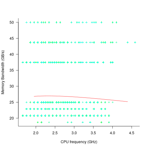
I was wrong. There does not appear to be any connection between a system’s cpu frequency and its memory bandwidth.
These days, most x86 chips include multiple processors, with each processor taking a share of memory bandwidth. Increasing memory bandwidth is essential, if all cores are to be kept busy.
The SPEC CPU benchmark measures the performance of a single processor. If only one of the cpu cores available on a system is being used, that core has the benefit of memory bandwidth that usually has to be shared.
To what extent is a single core benchmark relevant today? I suspect that most programs run on a single core, but developers sometimes attempt to spread cpu intensive programs over multiple cores. As always, data is needed.
The SPEC benchmark is useful for cpu designers (the original target market) and compiler writers wanting to measure the impact of fancy new optimizations.
Memory bandwidth: 1991-2009
The Stream benchmark is a measure of sustained memory bandwidth; the target systems are high performance computers. Sustained in the sense of distance running, rather than a short sprint (the term for this is peak memory bandwidth and occurs when the requested data is in cache), and bandwidth in the sense of bytes of memory read/written per second (implemented using chunks the size of a double precision floating-point type). The dataset contains 1,018 measurements collected between 1991 and 2009.
The dominant characteristic of high performance computing applications is looping over very large arrays, performing floating-point operations on all the elements. A fast floating-point arithmetic unit has to be connected to a memory subsystem that can keep it fed with new floating-point values and write back computed values.
The Stream benchmark, in Fortran and C, defines several arrays, each containing max(1e6, 4*size_of_available_cache) double precision floating-point elements. There are four loops that iterate over every element of the arrays, each loop containing a single statement; see Fortran code in the following table (q is a scalar, array elements are usually 8-bytes, with add/multiply being the floating-point operations):
Name Operation Bytes FLOPS Copy a(i) = b(i) 16 0 Scale a(i) = q*b(i) 16 1 Sum a(i) = b(i) + c(i) 24 1 Triad a(i) = b(i) + q*c(i) 24 2 |
A system’s memory bandwidth will depend on the speed of the DRAM chips, the performance of the devices that transport bytes to the cpu, and the ability of the cpu to handle incoming traffic. The Stream data contains 21 columns, including: the vendor, date, clock rate, number of cpus, kind of memory (i.e., shared/distributed), and the bandwidth in megabytes/sec for each of the operations listed above.
How does the measured memory bandwidth change over time?
For most of the systems, the values for each of Copy, Scale, Sum, and Triad are very similar. That the simplest statement, Copy, is sometimes a bit faster/slower than the most complicated statement, Triad, shows that floating-point performance is much smaller than the time taken to read/write values to memory; the performance difference is random variation.
Several fitted regression models explain over half of the variance in the data, with the influential explanatory variables being: clock speed, date, type of system (i.e., PC/Mac or something much more expensive). The plot below shows MB/sec for the Copy loop, with three fitted regression models (code+data):
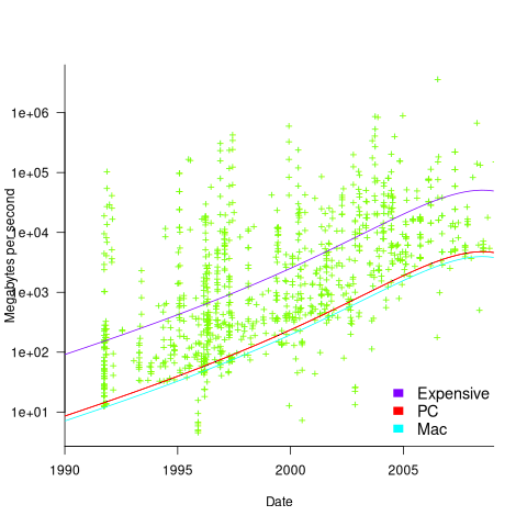
Fitting these models first required fitting a model for cpu clock rate over time; predictions of mean clock rate over time are needed as input to the memory bandwidth model. The three bandwidth models fitted are for PCs (189 systems), Macs (39 systems), and the more expensive systems (785; the five cluster systems were not fitted).
There was a 30% annual increase in memory bandwidth, with the average expensive systems having an order of magnitude greater bandwidth than PCs/Macs.
Clock rates stopped increasing around 2010, but go faster DRAM standards continue to be published. I assume that memory bandwidth continues to increase, but that memory performance is not something that gets written about much. The memory bandwidth on my new system is  MB/sec. This 2024 sample of one is 3.5 times faster than the average 2009 PC bandwidth, which is 100 times faster than the 1991 bandwidth.
The LINPACK benchmarks are the traditional application oriented cpu benchmarks used within the high performance computer community.
Techniques used for analyzing basic performance measurements
The statistical design and analysis of experiments is a relatively recent invention (around 150 years old; verifying scientific hypotheses using experiments was first proposed over 1,000 years ago).
Once an experiment has been run, and performance measurements collected, what techniques are available to analyse the data?
Before electronic computers were invented, the practical statistical techniques were those that could be performed manually (perhaps with some help from a mechanical calculator).
Once computers became available, these manual use techniques were widely implemented in statistical applications and libraries. New statistical techniques have been invented that are only of practical when a computer is available, e.g., the bootstrap.
Most researchers in software engineering remain stuck in the pre-computer world of statistical analysis, i.e., failing to use more powerful techniques that make use of computers. Software engineering is not unique in being stuck using pre-computer statistical techniques, there are many other fields that have failed to move on to the more flexible and powerful techniques now available.
Performance comparison by benchmarking (i.e., running an experiment) is a common activity in scientific and engineering fields. Once the measurements have been made, what is the difference between pre-computer and post-manual statistical comparison techniques?
Performance comparison invariably involves comparing the mean/average of each set of measurements (one set for each product benchmarked). Random variations will have some impact on the measured values, and it’s possible that any difference in mean values is the result of these random variations. There are statistical tests for estimating the likelihood of the difference being due to random variation.
Statistical tests invariably come with preconditions on the characteristics of their input data, i.e., the test only works as advertised if the preconditions are met.
The t.test is a popular pre-computer method of estimating the likelihood that the difference between the means of two sets of measurements occurred by chance. Two of its preconditions are that the two sets of input data have a Normal/Gaussian distribution, and have the same standard deviation (if the standard deviations are not equal, Welch’s t-test should be used).
The Mann–Whitney U test (also known as the Wilcoxon rank-sum test) is a pre-computer method with a more relaxed precondition on the distribution of the inputs, requiring only that they are drawn from the same distribution (which need not be a Normal distribution; it is a non-parametric test). This test returns the likelihood of one group being less/greater than the other, and says nothing about the magnitude of the difference.
Removing the constraint that it must be practical to manually perform the calculations, led, in 1979, to a paper proposing the Bootstrap (major issues around the theory underpinning the bootstrap were answered by the early 1990s).
The Bootstrap, a post-manual method, does not have any preconditions on the distribution or standard deviation of the input data. An important precondition is that it is reasonable to assume that the elements of the two sets of measurements are exchangeable (more on this below).
The Bootstrap is a general technique that is not limited to only comparing mean values, it can be used to compare any quantity of interest (assuming the appropriate data is available).
The bootstrap algorithm starts by assuming that, if the two samples are combined into an aggregate sample, all possible permutations of values in this aggregate into two samples are equally likely (this is the exchangeability assumption). If this assumption is true, then any compared difference in the measured two samples will be roughly the same as the compared difference in a pair of random samples drawn from the aggregate.
The computational intensive component of a bootstrap test is generating many pairs of random samples (5,000 is a common choice; sampling with replacement, and saving the result of the comparison).
The comparison results of the paired random samples and the two measured samples are sorted. The position of the measured comparison in this sorted list is the test statistic, i.e., how extreme is the result from the measured samples, compared to the random samples?
News of the flexibility and power of the bootstrap are slowly permeating through the research community. There is an existing way of doing things, and there is little incentive to change. As Plank famously observed: “Science advances one funeral at a time.”
Relative performance of computers from the 1950s/60s/70s
What was the range of performance of computers introduced in the 1950, 1960s and 1970s, and what was the annual rate of increase?
People have been measuring computer performance since they were first created, and thanks to the Internet Archive the published results are sometimes available today. The catch is that performance was often measured using different benchmarks. Fortunately, a few benchmarks were run on many systems, and in a few cases different benchmarks were run on the same system.
I have found published data on four distinct system performance estimation models, with each applied to 100+ systems (a total of 1,306 systems, of which 1,111 are unique). There is around a 20% overlap between systems across pairs of models, i.e., multiple models applied to the same system. The plot below shows the reported performance for pairs of estimates for the same system (code+data):

The relative performance relationship between pairs of different estimation models for the same system is linear (on a log scale).
Each of the models aims to produce a result that is representative of typical programs, i.e., be of use to people trying to decide which system to buy.
- Kenneth Knight built a structural model, based on 30 or so system characteristics, such as time to perform various arithmetic operations and I/O time; plugging in the values for a system produced a performance estimate. These characteristics were weighted based on measurements of scientific and commercial applications, to calculate a value that was representative of scientific or commercial operation. The Knight data appears in two magazine articles analysing systems from the 1950s and 1960s (the 310 rows are discussed in an earlier post), and the 1985 paper “A functional and structural measurement of technology”, containing data from the late 1960s and 1970s (120 rows),
- Ein-Dor and Feldmesser also built a structural model, based on the characteristics of 209 systems introduced between 1981 and 1984,
- The November 1980 Datamation article by Edward Lias lists what he called the KOPS (thousands of operations per second, i.e., MIPS for slower systems) value for 237 systems. Similar to the Knight and Ein-dor data, the calculated value is based on weighting various cpu instruction timings
- The Whetstone benchmark is based on running a particular program on a system, and recording its performance; this benchmark was designed to be representative of scientific and engineering applications, i.e., floating-point intensive. The design of this benchmark was the subject of last week’s post. I extracted 504 results from Roy Longbottom’s extensive collection of Whetstone results going back to the mid-1960s.
While the Whetstone benchmark was originally designed as an Algol 60 program that was representative of scientific applications written in Algol, only 5% of the results used this version of the benchmark; 85% of the results used the Fortran version. Fitting a regression model to the data finds that the Fortran version produced higher results than the Algol 60 version (which would encourage vendors to use the Fortran version). To ensure consistency of the Whetstone results, only those using the Fortran benchmark are used in this analysis.
A fifth dataset is the Dhrystone benchmark followed in the footsteps of the Whetstone benchmark, but targetting integer-based applications, i.e., no floating-point. First published in 1984, most of the Dhrystone results apply to more recent systems than the other benchmarks. This code+data contains the 328 results listed by the Performance Database Server.
Sometimes slightly different system names appear in the published results. I used the system names appearing in the Computers Models Database as the definitive names. It is possible that a few misspelled system names remain in the data (the possible impact is not matching systems up across models), please let me know if you spot any.
What is the best statistical technique to use to aggregate results from multiple models into a single relative performance value?
I came up with various possibilities, none of which looked that good, and even posted a question on Cross Validated (no replies yet).
Asking on the Evidence-based software engineering Discord channel produced a helpful reply from Neal Fultz, i.e., use the random effects model: lmer(log(metric) ~ (1|System)+(1|Bench), data=Sall_clean) ; after trying lots of other more complicated approaches, I would probably have eventually gotten around to using this approach.
Does this random effects model produce reliable values?
I don’t have a good idea how to evaluate the fitted model. Looking at pairs of systems where I know which is faster, the relative model values are consistent with what I know.
A csv of the calculated system relative performance values. I have yet to find a reliable way of estimating confidence bounds on these values.
The plot below shows the performance of systems introduced in a given year, on a relative scale, red line is a fitted exponential model (a factor of 5.5 faster, annually; code+data):
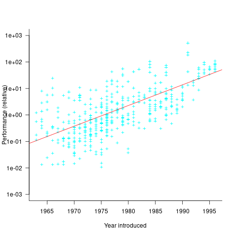
If you know of a more effective way of analysing this data, or any other published data on system benchmarks for these decades, please let me know.
Design of the Whetstone benchmark
The Whetstone benchmark was once a widely cited measure of computer performance. This benchmark consisted of a single program, originally designed for Algol 60 based applications, and later translated to other languages (over 85% of published results used Fortran). The source used as representative of typical user programs came from scientific applications, which has some characteristics that are very non-representative of non-scientific applications, e.g., use of floating-point, and proportionally more multiplications and multidimensional array accesses. Dhrystone benchmark was later designed with the intent of being representative of a broader range of applications.
While rooting around for Whetstone result data, I discovered the book Algol 60 Compilation and Assessment by Brian Wichmann. Despite knowing Brian for 25 years and being very familiar with his work on compiler validation, I had never heard of this book (Knuth’s An Empirical Study of Fortran Programs has sucked up all the oxygen in this niche).
As expected, this 1973 book has a very 1960s model of cpu/compiler behavior, much the same as MIX, the idealised computer used by Knuth for the first 30-years of The Art of Computer Programming.
The Whetstone world view is of a WYSIWYG compiler (i.e., each source statement maps to the obvious machine code), and cpu instructions that always take the same number of clock cycles to execute (the cpu/memory performance ratio had not yet moved far from unity, for many machines).
Compiler optimization is all about trying not to generate code, and special casing to eke out many small savings; post-1970 compilers tried hard not to be WYSIWYG. Showing compiler correctness is much simplified by WYSIWIG code generation.
Today, there are application domains where the 1960s machine model still holds. Low power embedded systems may have cpu/memory performance ratios close to unity, and predictable instruction execution times (estimating worst-case execution time is a minor research field).
Creating a representative usage-based benchmark requires detailed runtime data on what the chosen representative programs are doing. Brian modified the Whetstone Algol interpreter to count how many times each virtual machine op-code was executed (see the report Some Statistics from ALGOL Programs for more information).
The modified Algol interpreter was installed on the KDF9 at the National Physical Laboratory and Oxford University, in the late 1960s. Data from 949 programs was collected; the average number of operations per program was 152,000.
The op-codes need to be mapped to Algol statements, to create a benchmark program whose compiled form executes the appropriate proportion of op-codes. Some op-code sequences map directly to statements, e.g., Ld addrof x, Ld value y, Store, maps to the statement: x:=y;.
Counts of occurrences of each language construct in the source of the representative programs provides lots of information about the proportions of the basic building blocks. It’s ‘just’ a matter of sorting out the loop counts.
For me, the most interesting part of the book is chapter 2, which attempts to measure the execution time of 40+ different statements running on 36 different machines. The timing model is  , where
  is the
  ‘th statement,
  is the
  ‘th machine,
  an adjustment factor intended to be as close to one as possible, and
  is execution time. The book lists some of the practical issues with this model, from the analysis of timing data from current machines, e.g., the impact of different compilers, and particular architecture features having a big performance impact on some kinds of statements.
The table below shows statement execution time, in microseconds, for the corresponding computer and statement (* indicates an estimate; the book contains timings on 36 systems):
ATLAS MU5 1906A RRE Algol 68 B5500 Statement 6.0 0.52 1.4 14.0 12.1 x:=1.0 6.0 0.52 1.3 54.0 8.1 x:=1 6.0 0.52 1.4 *12.6 11.6 x:=y 9.0 0.62 2.0 23.0 18.8 x:=y + z 12.0 0.82 3.2 39.0 50.0 x:=y × z 18.0 2.02 7.2 71.0 32.5 x:=y/z 9.0 0.52 1.0 8.0 8.1 k:=1 18.0 0.52 0.9 121.0 25.0 k:=1.0 12.0 0.62 2.5 13.0 18.8 k:=l + m 15.0 1.07 4.9 75.0 35.0 k:=l × m 48.0 1.66 6.7 45.0 34.6 k:=l ÷ m 9.0 0.52 1.9 8.0 11.6 k:=l 6.0 0.72 3.1 44.0 11.8 x:=l 18.0 0.72 8.0 122.0 26.1 l:=y 39.0 0.82 20.3 180.0 46.6 x:=y ^ 2 48.0 1.12 23.0 213.0 85.0 x:=y ^ 3 120.0 10.60 55.0 978.0 1760.0 x:=y ^ z 21.0 0.72 1.8 22.0 24.0 e1[1]:=1 27.0 1.37 1.9 54.0 42.8 e1[1, 1]:=1 33.0 2.02 1.9 106.0 66.6 e1[1, 1, 1]:=1 15.0 0.72 2.4 22.0 23.5 l:=e1[1] 45.0 1.74 0.4 52.0 22.3 begin real a; end 96.0 2.14 80.0 242.0 2870.0 begin array a[1:1]; end 96.0 2.14 86.0 232.0 2870.0 begin array a[1:500]; end 156.0 2.96 106.0 352.0 8430.0 begin array a[1:1, 1:1]; end 216.0 3.46 124.0 452.0 13000.0 begin array a[1:1, 1:1, 1:1]; end 42.0 1.56 3.5 16.0 31.5 begin goto abcd; abcd : end 129.0 2.08 9.4 62.0 98.3 begin switch s:=q; goto s[1]; q : end 210.0 24.60 73.0 692.0 598.0 x:=sin(y) 222.0 25.00 73.0 462.0 758.0 x:=cos(y) 84.0 *0.58 17.3 22.0 14.0 x:=abs(y) 270.0 *10.20 71.0 562.0 740.0 x:=exp(y) 261.0 *7.30 24.7 462.0 808.0 x:=ln(y) 246.0 *6.77 73.0 432.0 605.0 x:=sqrt(y) 272.0 *12.90 91.0 622.0 841.0 x:=arctan(y) 99.0 *1.38 18.7 72.0 37.5 x:=sign(y) 99.0 *2.70 24.7 152.0 41.1 x:=entier(y) 54.0 2.18 43.0 72.0 31.0 p0 69.0 *6.61 57.0 92.0 39.0 p1(x) 75.0 *8.28 65.0 132.0 45.0 p2(x, y) 93.0 *9.75 71.0 162.0 53.0 p2(x, y, z) 57.0 *0.92 8.6 17.0 38.5 loop time |
The performance studies found wide disparities between expected and observed timings. Chapter 9 does a deep dive on six Algol compilers.
A lot of work and idealism went into gather the data for this book (36 systems!). Unfortunately, the computer performance model was already noticeably inaccurate, and advances in compiler optimization and cpu design meant that the accuracy was only going to get worse. Anyways, there is lots of interesting performance data on 1960 era computers.
Whetstone lived on into the 1990s, when the SPEC benchmark started to its rise to benchmark dominance.
Benchmarking fuzzers
Fuzzing has become a popular area of research in the reliability & testing community, with a stream of papers claiming to have created a better tool/algorithm. The claims of ‘betterness’, made by the authors, often derive from the number of previously unreported faults discovered in some collection of widely used programs.
Developers in industry will be interested in using fuzzing if it provides a cost-effective means of discovering coding mistakes that are likely to result in customers experiencing a serious fault. This requirement roughly translates to: minimal cost for finding maximal distinct mistakes (finding the same mistake more than once is wasted effort); whether a particular coding mistake is likely to produce a serious customer fault is a decision decided by people.
How do different fuzzing tools compare, when benchmarking the number of distinct mistakes they each find, for a given amount of cpu time?
TL;DR: I don’t know, and this approach is probably not a useful way of comparing fuzzers.
Fuzzing researchers are currently competing on the number of previously unreported faults discovered, i.e., not listed in the fuzzed program’s database of fault reports. Most research papers only report the number of distinct faults discovered in each program fuzzed, the amount of wall clock hours/days used (sometimes weeks), and the characteristics of the computer/cluster on which the campaign was run. This may be enough information to estimate an upper bound on faults per unit of cpu time; more detailed data is rarely available (I have emailed the authors of around a dozen papers asking for more detailed data).
A benchmark based on comparing faults discovered per unit of cpu time only makes sense when the new fault discovery rate is roughly constant. Experience shows that discovery time can vary by orders of magnitude.
Code coverage is a fuzzer performance metric that is starting to be widely used by researchers. Measures of coverage include: statements/basic blocks, conditions, or some object code metric. Coverage has the advantage of providing defined fuzzer objectives (e.g., generate input that causes uncovered code to be executed), and is independent of the number of coding mistakes present in the code.
How is a fuzzer likely to be used in industry?
The fuzzing process may be incremental, discovering a few coding mistakes, fixing them, rinse and repeat; or, perhaps fuzzing is run in a batch over, say, a weekend when the test machine is available.
The current research approach is batch based, not fixing any of the faults discovered (earlier researchers fixed faults).
Not fixing discovered faults means that underlying coding mistakes may be repeatedly encountered, which wastes cpu time because many fuzzers terminate the run when the program they are testing crashes (a program crash is a commonly encountered fuzzing fault experience). The plot below shows the number of occurrences of the same underlying coding mistake, when running eight fuzzers on the program JasPer; 77 distinct coding mistakes were discovered, with three fuzzers run over 3,000 times, four run over 1,500 times, and one run 62 times (see Green Fuzzing: A Saturation-based Stopping Criterion using Vulnerability Prediction by Lipp, Elsner, Kacianka, Pretschner, Böhme, and Banescu; code+data):
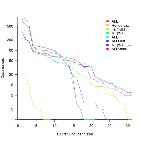
I have not seen any paper where the researchers attempt to reduce the number of times the same root cause coding mistake is discovered. Researchers are focused on discovering unreported faults; and with around 98% of fault discoveries being duplicates, appear to have resources to squander.
If developers primarily use a find/fix iterative process, then duplicate discoveries will be an annoying drag on cpu time. However, duplicate discoveries are going to make it difficult to effectively benchmark fuzzers.
WebAssembly vs JavaScript performance: 2023 edition
WebAssembly is an assembly-like language intended to be executed by web browsers on an internal stack machine. The intent is that compilers for high-level languages (i.e., C, Cobol, and C#) treat WebAssembly just like they would the assembly language of a cpu. Some substantial applications have been ported, e.g., the R statistical environment, which is written in C and Fortran.
Some people claim that WebAssembly based applications will run faster, and consume less power, than those written in JavaScript or PHP. Now, one virtual machine is as much like any other. Performance differences are driven by compiler optimizations, the ease with which particular language features can be mapped to the available instructions, and an application’s use of easy/hard to map high-level language features.
Researchers have run benchmarks to compare the runtime performance and power consumption of Wasm against other browser based languages, and this post analyses the runtime performance results from two papers.
TL;DR: Relative performance for Wasm/JavaScript varies across browsers and programs. Everything interacts with everything else, which makes analysis complicated.
As is the case with most data analysis in software engineering, the researchers used rudimentary statistical techniques (which is a shame given the huge effort that went into collecting the data). The conclusions of both papers is that for WebAssembly/JavaScript, relative performance issues are complicated, but the techniques they used did not enable them to understand why.
What kind of statistical techniques are applicable for analysing these benchmarks?
Use of different languages/browsers might be expected to have some percentage impact on performance, e.g., programs written in language X will be p% faster/slower. The following equation is one modelling approach, and this equation can be fitted using nonlinear regression:
(1+c_j Browser_j)") , where:
, where:  is a constant,
  is the fitted constant for language
  , and
, and  is the fitted constant for browser
The problem with this equation is that it involves a separate equation for each combination of language/browser (assuming that all benchmarks are bundled together in the value of ). It is possible to use a single equation when there are just two languages/two browsers, by mapping them to the values 0/1.
All languages/browsers/benchmarks can be included in a single linear regression model by treating them as factors in a log transformed model; the equation is:  , where:
  is the fitted constant for benchmark
  . The values of , , and are zero, or one for the corresponding fitted constant. All the factors on the right-hand-side are discrete, so a log transform has nothing to distort.
The fitted equation can then be transformed to:

This model assumes that each factor is independent of the others, i.e., the relative performance of each language does not depend on the browser, and that relative performance does not significantly vary between benchmarks, e.g., if  runs 10% faster when implemented in
  , then
  also runs close to 10% faster when implemented in .
How well did the benchmark data from the two papers fit this model, and what were the performance numbers?
The study WebAssembly versus JavaScript: Energy and Runtime Performance by De Macedo, Abreu, Pereira, and Saraiva ran a wide range of benchmarks. It compared C/Wasm/JavaScript running on Chrome/Firefox/Edge. One set of benchmarks were 10 small compute-intensive programs (in Wasm/JavaScript), which were executed with small/medium/large amounts of input data; the other set of benchmarks were two large applications WasmBoy is a Game-boy/Gameboy Color Emulator (written in Typescript and compiled to Wasm), and PSPDFKit supporting viewing, annotating, and filling in forms in PDF documents (written in C/C++ and compiled to a both a subset of JavaScript and Wasm).
Results from the 10 small benchmarks showed strong interactions between browser and language (i.e., Wasm performance relative to JavaScript, varied between browsers; with Edge being faster and Firefox being slower), and a lot of interaction between benchmark and input data size. Support for Wasm is relatively new, relative to the much more mature JavaScript, so it’s not surprising that different browsers have different performance; I’m arm waving when I say that the input size dependency may be related to JIT issues (code).
When interactions are included, the fitted equation has the form:

Analysing the results for the two applications, we find that:
- WasmBoy: the factors were independent, and WebAssembly was faster than JavaScript. The
 factor was 0.84 for Wasm and 1 for JavaScript,
 - PSPDFKit: there was interaction between the language and browser, with behavior similar to that seen for the small benchmarks.
The study Comparing the Energy Efficiency of WebAssembly and JavaScript in Web Applications on Android Mobile Devices by van Hasselt, Huijzendveld, Noort, de Ruijter, Islam, and Malavolta compared the performance of WebAssembly/JavaScript running compute intensive benchmarks on Firefox/Chrome.
Fitting a regression model to the data from the eight benchmarks showed strong interactions between benchmark programs and language, with each language being faster for some programs (code).
It’s not surprising that the results failed to show a conclusive performance advantage for either WebAssembly or JavaScript, across benchmarks. The situation might change as the wasm virtual machine is tuned, and compilers targetting wasm implement a wider range of optimizations.
Update
A performance analysis of C, Rust, Go, and Javascript compiled to Webassembler
A comparison of C++ and Rust compiler performance
Large code bases take a long time to compile and build. How much impact does the choice of programming language have on compiler/build times?
The small number of industrial strength compilers available for the widely used languages makes the discussion as much about distinct implementations as distinct languages. And then there is the issue of different versions of the same compiler having different performance characteristics; for instance, the performance of Microsoft’s C++ Visual Studio compiler depends on the release of the compiler and the version of the standard specified.
Implementation details can have a significant impact on compile time. Compile time may be dominated by lexical analysis, while support for lots of fancy optimization shifts the time costs to code generation, and poorly chosen algorithms can result in symbol table lookup being a time sink (especially for large programs). For short programs, compile time may be dominated by start-up costs. These days, developers rarely have to worry about small memory size causing occurring when compiling a large source file.
A recent blog post compared the compile/build time performance of Rust and C++ on Linux and Apple’s OS X, and strager kindly made the data available.
The most obvious problem with attempting to compare the performance of compilers for different languages is that the amount of code contained in programs implementing the same functionality will differ (this is also true when the programs are written in the same language).
strager’s solution was to take a C++ program containing 9.3k LOC, plus 7.3K LOC of tests, and convert everything to Rust (9.5K LOC, plus 7.6K LOC of tests). In total, the benchmark consisted of compiling/building three C++ source files and three equivalent Rust source files.
The performance impact of number of lines of source code was measured by taking the largest file and copy-pasting it 8, 16, and 32 times, to create three every larger versions.
The OS X benchmarks did not include multiple file sizes, and are not included in the following analysis.
A variety of toolchain options were included in different runs, and for Rust various command line options; most distinct benchmarks were run 10 times each. On Linux, there were a total of 360 C++ runs, and for Rust 1,066 runs (code+data).
The model  , where
  is a fitted regression constant, and
  is the fitted regression coefficient for the ‘th benchmark, explains just over 50% of the variance. The language is implicit in the benchmark information.
The model -0.84L}") , where
, where  is the number of copies,
  is 0 for C++ and 1 for Rust, explains 92% of the variance, i.e., it is a very good fit.
The expression -0.84L}") is a language and source code size multiplication factor. The numeric values are:
is a language and source code size multiplication factor. The numeric values are:
1 8 16 32 C++ 1.03 1.25 1.57 2.45 Rust 0.98 1.52 2.52 6.90 |
showing that while Rust compilation is faster than C++, for ‘shorter’ files, it becomes much relatively slower as the quantity of source increases.
The size factor for Rust is growing quadratically, while it is much closer to linear for C++.
What are the threats to the validity of this benchmark comparison?
The most obvious is the small number of files benchmarked. I don’t have any ideas for creating a larger sample.
How representative is the benchmark of typical projects? An explicit goal in benchmark selection was to minimise external dependencies (to reduce the effort likely to be needed to translate to Rust). Typically, projects contain many dependencies, with compilers sometimes spending more time processing dependency information than compiling the actual top-level source, e.g., header files in C++.
A less obvious threat is the fact that the benchmarks for each language were run in contiguous time intervals, i.e., all Rust, then all C++, then all Rust (see plot below; code+data):
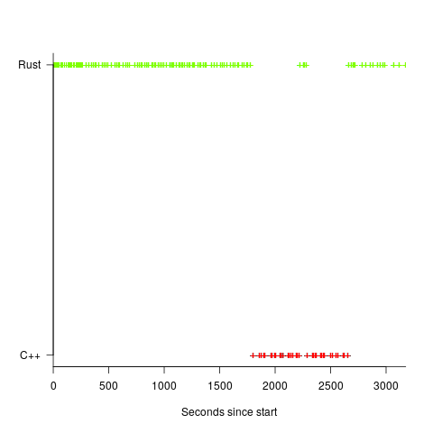
It is possible that one or more background processes were running while one set of language benchmarks was being run, which would skew the results. One solution is to intermix the runs for each language (switching off all background tasks is much harder).
I was surprised by how well the regression model fitted the data; the fit is rarely this good. Perhaps a larger set of benchmarks would increase the variance.
Recent Comments