Archive
Fitting discontinuous data from disparate sources
Sorting and searching are probably the most widely performed operations in computing; they are extensively covered in volume 3 of The Art of Computer Programming. Algorithm performance is influence by the characteristics of the processor on which it runs, and the size of the processor cache(s) has a significant impact on performance.
A study by Khuong and Morin investigated the performance of various search algorithms on 46 different processors. Khuong The two authors kindly sent me a copy of the raw data; the study webpage includes lots of plots.
The performance comparison involved 46 processors (mostly Intel x86 compatible cpus, plus a few ARM cpus) times 3 array datatypes times 81 array sizes times 28 search algorithms. First a 32/64/128-bit array of unsigned integers containing N elements was initialized with known values. The benchmark iterated 2-million times around randomly selecting one of the known values, and then searching for it using the algorithm under test. The time taken to iterate 2-million times was recorded. This was repeated for the 81 values of N, up to 63,095,734, on each of the 46 processors.
The plot below shows the results of running each algorithm benchmarked (colored lines) on an Intel Atom D2700 @ 2.13GHz, for 32-bit array elements; the kink in the lines occur roughly at the point where the size of the array exceeds the cache size (all code+data):

What is the most effective way of analyzing the measurements to produce consistent results?
One approach is to build two regression models, one for the measurements before the cache ‘kink’ and one for the measurements after this kink. By adding in a dummy variable at the kink-point, it is possible to merge these two models into one model. The problem with this approach is that the kink-point has to be chosen in advance. The plot shows that the performance kink occurs before the array size exceeds the cache size; other variables are using up some of the cache storage.
This approach requires fitting 46*3=138 models (I think the algorithm used can be integrated into the model).
If data from lots of processors is to be fitted, or the three datatypes handled, an automatic way of picking where the first regression model should end, and where the second regression model should start is needed.
Regression discontinuity design looks like it might be applicable; treating the point where the array size exceeds the cache size as the discontinuity. Traditionally discontinuity designs assume a sharp discontinuity, which is not the case for these benchmarks (R’s rdd package worked for one algorithm, one datatype running on one processor); the more recent continuity-based approach supports a transition interval before/after the discontinuity. The R package rdrobust supports a continued-based approach, but seems to expect the discontinuity to be a change of intercept, rather than a change of slope (or rather, I could not figure out how to get it to model a just change of slope; suggestions welcome).
Another approach is to use segmented regression, i.e., one of more distinct lines. The package segmented supports fitting this kind of model, and does estimate what they call the breakpoint (the user has to provide a first estimate).
I managed to fit a segmented model that included all the algorithms for 32-bit data, running on one processor (code+data). Looking at the fitted model I am not hopeful that adding data from more than one processor would produce something that contained useful information. I suspect that there are enough irregular behaviors in the benchmark runs to throw off fitting quality.
I’m always asking for more data, and now I have more data than I know how to analyze in a way that does not require me to build 100+ models 🙁
Suggestions welcome.
Benchmarking desktop PCs circa 1990
Before buying a computer customers want to be confident of choosing the best they can get for the money, and performance has often been a major consideration. Computer benchmark performance results were once widely discussed.
Knight’s analysis of early mainframe performance was widely cited for many years.
Performance on the Byte benchmarks was widely cited before Intel started spending billions on advertising, clock frequency has not always had the brand recognition it has today.
The Byte benchmark was originally designed for Intel x86 processors running Microsoft DOS; The benchmark was introduced in the June 19885 issue, and was written in the still relatively new C language (earlier microprocessor benchmarks were often written in BASIC, because early micros often came with a free BASIC interpreter), it was updated in the 1990s to be Windows based, and implemented for Unix.
Benchmarking computers using essentially the same cpu architecture and operating system removes many complications that have to be addressed when these differ. Before Wintel wiped them out, computers from different manufacturers (and often the same manufacturer) contained completely different cpu architectures, ran different operating systems, and compilers were usually created in-house by the manufacturer (or some university who got a large discount on their computer purchase).
The Fall 1990 issue of Byte contains tables of benchmark results from 1988-90. What can we learn from these results?
The most important takeaway from the tables is that those performing the benchmarks appreciated the importance of measuring hardware performance using the applications that customers are likely to be running on their computer, e.g., word processors, spreadsheets, databases, scientific calculations (computers were still sufficiently niche back then that scientific users were a non-trivial percentage of the market), and compiling (hackers were a large percentage of Byte’s readership).
The C benchmarks attempted to measure CPU, FPU (built-in hardware support for floating-point arrived with the 486 in April 1989, prior to that it was an add-on chip that required spending more money), Disk and Video (at the time support for color was becoming mainstream, but bundled hardware graphics support still tended to be minimal).
Running the application benchmarks takes a lot of time, plus the necessary software (which takes time to install from floppies, the distribution technology of the day). Running the C benchmarks is much quicker and simpler.
Ideally the C benchmarks are a reliable stand-in for the application benchmarks (meaning that only the C benchmarks need be run).
Let’s fit some regression models to the measurements of the 61 systems benchmarked, all supporting hardware floating-point (code+data). Surprisingly there is no mention of such an exercise being done by the Byte staff, even though one of the scientific benchmarks included regression fitting.
The following fitted equations explain around 90% of the variance of the data, i.e., they are good fits.

For word-processing, the CPU benchmark explains around twice as much as the Disk benchmark.

For spreadsheets, CPU and Disk contribute about the same.

Database is nearly all Disk.
+0.45*CPU*Disk")
Scientific/Engineering is FPU, plus interactions with other components.
+0.33*Disk*Video")
Compiling is CPU, plus interactions with other components.
Byte’s benchmark reports were great eye candy, and readers probably took away a rough feel for the performance of various systems. Perhaps somebody at the time also fitted regression models to the data. The magazine contained plenty of adverts for software to do this.
Modeling visual studio C++ compile times
Last week I spotted an interesting article on the compile-time performance of C++ compilers running under Microsoft Windows. The author had obviously put a lot of work into gathering the data, and had taken care to have multiple runs to reduce the impact of random effects (128 runs to be exact); but, as if often the case, the analysis of the data was lackluster. I posted a comment asking for the data, and a link was posted the next day 🙂
The compilers benchmarked were: Visual Studio 2015, Visual Studio 2017 and clang 7.0.1; the compilers were configured to target: C++20, C++17, C++14, C++11, C++03, or C++98. The source code used was 100 system headers.
If we are interested in understanding the contribution of each component to overall compile-time, the obvious fist regression model to build is:

where:  are the different headers,
  the different compilers and
  the different target languages. There might be some interaction between variables, so something more complicated was tried first; the final fitted model was (code+data):

where  is a constant (the
 Intercept in R’s summary output). The following is a list of normalised numbers to plug into the equation (clang is the default compiler and C++03 the default language, and so do not appear in the list, the : symbol represents the multiplication; only a few of the 100 headers are listed, details are available):
Estimate Std. Error t value Pr(>|t|) (Intercept) headerany 1.000000000 0.051100398 headerarray headerassert.h 0.522336397 -0.654056185 ... headerwctype.h headerwindows.h -0.648095154 1.304270250 compilerVS15 compilerVS17 -0.185795534 -0.114590143 languagec++11 languagec++14 0.032930014 0.156363433 languagec++17 languagec++20 0.192301727 0.184274629 languagec++98 compilerVS15:languagec++11 0.001149643 -0.058735591 compilerVS17:languagec++11 compilerVS15:languagec++14 -0.038582437 -0.183708714 compilerVS17:languagec++14 compilerVS15:languagec++17 -0.164031495 NA compilerVS17:languagec++17 compilerVS15:languagec++20 -0.181591418 NA compilerVS17:languagec++20 compilerVS15:languagec++98 -0.193587045 0.062414667 compilerVS17:languagec++98 0.014558295 |
As an example, the (normalised) time to compile wchar.h using VS15 with languagec++11 is:
1-0.514807638-0.183862162+0.033951731-0.059720131
Each component adds/substracts to/from the normalised mean.
Building this model didn’t take long. While waiting for the kettle to boil, I suddenly realised that an additive model was probably inappropriate for this problem; oops. Surely the contribution of each component was multiplicative, i.e., components have a percentage impact to performance.
A quick change to the form of the fitted model:
 = k+header_x+compiler_y+language_z+compiler_y*language_z")
Taking the exponential of both side, the fitted equation becomes:

The numbers, after taking the exponent, are:
(Intercept) headerany 9.724619e+08 1.051756e+00 ... headerwctype.h headerwindows.h 3.138361e-01 2.288970e+00 compilerVS15 compilerVS17 7.286951e-01 7.772886e-01 languagec++11 languagec++14 1.011743e+00 1.049049e+00 languagec++17 languagec++20 1.067557e+00 1.056677e+00 languagec++98 compilerVS15:languagec++11 1.003249e+00 9.735327e-01 compilerVS17:languagec++11 compilerVS15:languagec++14 9.880285e-01 9.351416e-01 compilerVS17:languagec++14 compilerVS15:languagec++17 9.501834e-01 NA compilerVS17:languagec++17 compilerVS15:languagec++20 9.480678e-01 NA compilerVS17:languagec++20 compilerVS15:languagec++98 9.402461e-01 1.058305e+00 compilerVS17:languagec++98 1.001267e+00 |
Taking the same example as above: wchar.h using VS15 with c++11. The compile-time (in cpu clock cycles) is:
9.724619e+08*3.138361e-01*7.286951e-01*1.011743e+00*9.735327e-01
Now each component causes a percentage change in the (mean) base value.
Both of these model explain over 90% of the variance in the data, but this is hardly surprising given they include so much detail.
In reality compile-time is driven by some combination of additive and multiplicative factors. Building a combined additive and multiplicative model is going to be like wrestling an octopus, and is left as an exercise for the reader 🙂
Given a choice between these two models, I think the multiplicative model is probably closest to reality.
Building a regression model is easy and informative
Running an experiment is very time-consuming. I am always surprised that people put so much effort into gathering the data and then spend so little effort analyzing it.
The Computer Language Benchmarks Game looks like a fun benchmark; it compares the performance of 27 languages using various toy benchmarks (they could not be said to be representative of real programs). And, yes, lots of boxplots and tables of numbers; great eye-candy, but what do they all mean?
The authors, like good experimentalists, make all their data available. So, what analysis should they have done?
A regression model is the obvious choice and the following three lines of R (four lines if you could the blank line) build one, providing lots of interesting performance information:
cl=read.csv("Computer-Language_u64q.csv.bz2", as.is=TRUE)

cl_mod=glm(log(cpu.s.) ~ name+lang, data=cl)
summary(cl_mod) |
The following is a cut down version of the output from the call to summary, which summarizes the model built by the call to glm.
                    Estimate Std. Error t value Pr(>|t|)
(Intercept)         1.299246   0.176825   7.348 2.28e-13 ***
namechameneosredux  0.499162   0.149960   3.329 0.000878 ***
namefannkuchredux   1.407449   0.111391  12.635  < 2e-16 ***
namefasta           0.002456   0.106468   0.023 0.981595
namemeteor         -2.083929   0.150525 -13.844  < 2e-16 ***

langclojure         1.209892   0.208456   5.804 6.79e-09 ***
langcsharpcore      0.524843   0.185627   2.827 0.004708 **
langdart            1.039288   0.248837   4.177 3.00e-05 ***
langgcc            -0.297268   0.187818  -1.583 0.113531
langocaml          -0.892398   0.232203  -3.843 0.000123 ***

    Null deviance: 29610  on 6283  degrees of freedom
Residual deviance: 22120  on 6238  degrees of freedom
What do all these numbers mean?
We start with glm's first argument, which is a specification of the regression model we are trying to fit: log(cpu.s.) ~ name+lang
cpu.s. is cpu time, name is the name of the program and lang is the language. I found these by looking at the column names in the data file. There are other columns in the data, but I am running in quick & simple mode. As a first stab, I though cpu time would depend on the program and language. Why take the log of the cpu time? Well, the model fitted using cpu time was very poor; the values range over several orders of magnitude and logarithms are a way of compressing this range (and the fitted model was much better).
The model fitted is:
 , or
, or 
Plugging in some numbers, to predict the cpu time used by say the program chameneosredux written in the language clojure, we get:  (values taken from the first column of numbers above).
This model assumes there is no interaction between program and language. In practice some languages might perform better/worse on some programs. Changing the first argument of glm to: log(cpu.s.) ~ name*lang, adds an interaction term, which does produce a better fitting model (but it's too complicated for a short blog post; another option is to build a mixed-model by using lmer from the lme4 package).
We can compare the relative cpu time used by different languages. The multiplication factor for clojure is  , while for
 ocaml it is  . So
. So clojure consumes 8.2 times as much cpu time as ocaml.
How accurate are these values, from the fitted regression model?
The second column of numbers in the summary output lists the estimated standard deviation of the values in the first column. So the clojure value is actually }") , i.e., between 2.2 and 4.9 (the multiplication by 1.96 is used to give a 95% confidence interval); the
, i.e., between 2.2 and 4.9 (the multiplication by 1.96 is used to give a 95% confidence interval); the ocaml values are }") , between 0.3 and 0.6.
, between 0.3 and 0.6.
The fourth column of numbers is the p-value for the fitted parameter. A value of lower than 0.05 is a common criteria, so there are question marks over the fit for the program fasta and language gcc. In fact many of the compiled languages have high p-values, perhaps they ran so fast that a large percentage of start-up/close-down time got included in their numbers. Something for the people running the benchmark to investigate.
Isn't it easy to get interesting numbers by building a regression model? It took me 10 minutes, ok I spend a lot of time fitting models. After spending many hours/days gathering data, spending a little more time learning to build simple regression models is well worth the effort.
Cost/performance analysis of 1944-1967 computers: Knight’s data
Changes In Computer Performance and Evolving Computer Performance 1963-1967, by Kenneth Knight, are the references to cite when discussing the performance of early computers. I suspect that very few people have read the two papers they are citing (citing without reading is a surprisingly common practice). Both papers were published in Datamation, a computer magazine whose technical contents could rival that of the ACM journals in the 1960s, but later becoming more of a trade magazine. Until the articles appeared on bitsavers.org they were only really available through national or major regional libraries.
Both papers contain lots of interesting performance and cost data on computers going back to the 1940s. However, I was not interested enough to type in all that data. This week I found high quality OCRed copies of the papers on the Internet Archive; my effort was reduced to fixing typos, which felt like less work.
So let’s try to reproduce Knight’s analysis of the data (code and data). Working in the mid-1960s, I imagine Knight did everything manually, with the help of mechanical calculators. I have the advantage of fancy software, a very fast computer and techniques that were invented after Knight did his analysis (e.g., generalized linear methods).
Each paper contains its own dataset: the first contains performance+cost data on 225 computers available between 1944 and 1963, while the second contains this information on 63 computers available between 1963 and 1967.
The dataset lists the computer name, the date it was introduced, number of operations per second and the number of seconds that can be rented for a dollar (most computer time used to be rented, then 25 years later personal computers came along and people got to own one, now, 25 years after that Cloud is causing a switch back to rental per second).
How are operations measured? The MIPS unit of measurement did not start to be generally used until the 1980s. Knight used 30 or so system characteristics, such as time to perform various arithmetic operations and I/O time, plus characteristics of scientific and commercial applications to calculate a value considered to be a representative scientific or commercial operation.
There is no mention of how seconds-per-dollar values were obtained. Did Knight ask customers or vendors? In a rental market, I imagine vendor pricing could be very flexible.
In the 1970s people started talking about Moore’s law, but in the 1960s there was Grosch’s law: Computer performance increases as the square of the cost, i.e., faster computers were cheaper to rent, for a given number of operations. Knight set out to empirically check Grosch’s law, i.e., he was looking for a quadratic fit.
Fitting a regression model to the 1950-1961 data, Knight obtained an exponent of 2.18, while I obtained 2.38 for commercial operations (using a slightly more sophisticated model, because I could); time on faster computers was cheaper than Grosch claimed. For scientific operations, Knight obtained 1.92, while I obtained 3.56; despite trying all sorts of jiggery-pokery I could not get a lower value. Unless Knight used very different values to the ones published in the ‘scientific’ columns, one of us has made a big mistake (please let me know if my code is wrong).
Fitting a regression model to the 1963-1967 data, I get figures (both around 2.85 and 2.94) that are roughly in agreement with Knight (2.5 and 3.1). Grosch’s law has broken down by 1963 (if it ever held for scientific operations).
The plot below shows operations per second against operationsseconds per dollar for the 1953-1961 data, with fitted lines for some specific years. It shows that while customers get fewer seconds per dollar on faster computers, the number of operations performed in those seconds is raised to the power of two+ (code and data):
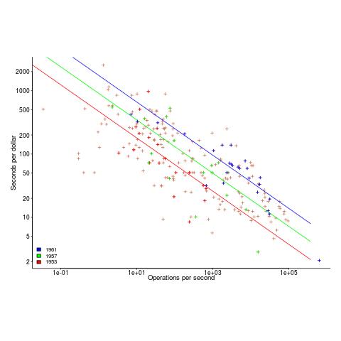
What other information can be extracted from the data? The 1953-1961 data shows seconds per dollar increased, over the whole performance range, by a factor of 1.15 per year, i.e., 15%, for both scientific and commercial; the 1963-1967 year-on-year increase jumps around a lot.
Peak memory transfer rate is best SPECint performance predictor
The idea that cpu clock rate is the main driver of system performance on the SPEC2006 cpu benchmark is probably well entrenched in developers’ psyche. Common knowledge, or folklore, is slow to change. The apparently relentless increase in cpu clock rate, a side-effect of Moore’s law, stopped over 10 years ago, but many developers still behave as-if it is still happening today.
The plot below shows the SPEC cpu integer performance of 4,332 systems running at various clock rates; the colors denote the different peak memory transfer rates of the memory chips in these systems (code and data).
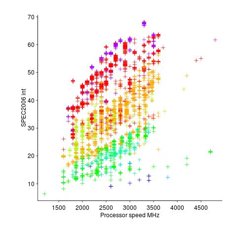
Fitting a regression model to this data, we find that the following equation predicts 80% of the variance (more complicated models fit better, but let’s keep it simple):

where: Processor.MHz is the processor clock rate, memrate the peak memory transfer rate and memfreq the frequency at which the memory is clocked.
Analysing the relative contribution of each of the three explanatory variables turns up the surprising answer that peak memory transfer rate explains significantly more of the variation in the data than processor clock rate (by around a factor of five).
If you are in the market for a new computer and are interested in relative performance, you can obtain a much more accurate estimate of performance by using the peak memory transfer rate of the DIMMs contained in the various systems you were considering. Good luck finding out these numbers; I bet the first response to your question will be “What is a DIMM?”
Developer focus on cpu clock rate is no accident, there is one dominant supplier who is willing to spend billions on marketing, with programs such as Intel Inside and rebates to manufacturers for using their products. There is no memory chip supplier enjoying the dominance that Intel has in cpus, hence nobody is willing to spend the billions in marketing need to create customer awareness of the importance of memory performance to their computing experience.
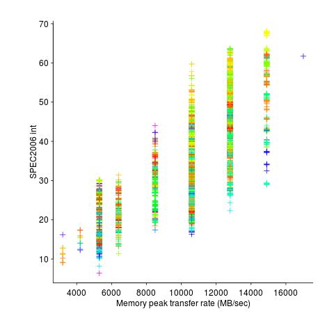
The plot below shows the SPEC cpu integer performance against peak memory transfer rates; the colors denote the different cpu clock rates in these systems.
Changes in optimization performance of gcc over time
The SPEC benchmarks came out a year after the first release of gcc (in fact gcc was and still is one of the programs included in the benchmark). Compiling the SPEC programs using the gcc option -O2 (sometimes -O3) has always been the way to measure gcc performance, but after 25 years does this way of doing things tell us anything useful?
The short answer: No
The longer answer is below as another draft section from my book Empirical software engineering with R book. As always comments welcome.
Changes in optimization performance of gcc over time
The GNU Compiler Collection <book gcc-man_12> (GCC) is under active development with its most well known component, the C compiler gcc, now over 25 years old. After such a long period of development is the quality of code generated by gcc still improving and if so at what rate? The method typically used to measure compiler performance is to compile the [SPEC] benchmarks with a small set of optimization options switched on (e.g., the O2 or O3 options) and this approach is used for the analysis performed here.
Data
Vladimir N. Makarow measured the performance of 9 releases of gcc, occurring between 2003 and 2010, on the same computer using the same benchmark suite (SPEC2000); this data is used in the following analysis.
The data contains the [SPEC number] (i.e., runtime performance) and code size measurements on 12 integer programs (11 in C and one in C+\+) from SPEC2000 compiled with gcc versions 3.2.3, 3.3.6, 3.4.6, 4.0.4, 4.1.2, 4.2.4, 4.3.1, 4.4.0 and 4.5.0 at optimization levels O2 and O3 (the mtune=pentium4 option was also used) 32-bit for the Intel Pentium 4 processor.
The same integer programs and 14 floating-point programs (10 in Fortran and 4 in C) were compiled for 64-bits, again with the O2 and O3 options (the mpc64 floating-point option was also used), using gcc versions 4.0.4, 4.1.2, 4.2.4, 4.3.1, 4.4.0 and 4.5.0.
Is the data believable?
The following are two fitness-for-purpose issues associated with using programs from SPEC2000 for these measurements:
-
the benchmark is designed for measuring processor performance not
compiler performance, -
many of its programs have been used for compiler benchmarking for
many years and it is likely that gcc has already been tuned to do
well on this benchmark.
The runtime performance measurements were obtained by running each programs once, SPEC requires that each program be run three times and the middle one chosen. Multiple measurements of each program would have increased confidence in their accuracy.
Predictions made in advance
Developers continue to make improvements to gcc and it is hoped that its optimization performance is increasing, knowing that performance is at a steady state or decreasing performance is also of interest.
No hypothesis is proposed for how optimization performance, as measured by the O2 and O3 options, might change between releases of gcc over the period 2003 to 2010.
The gcc documentation says that using the O3 option causes more optimizations to be performed than when the O2 option is used and therefore we would expect better performance for programs compiled with O3.
Applicable techniques
Modelling individual O2 and O3 option performance
One technique for modelling changes in optimization performance is to build a linear model that fits the gcc version (i.e., version is the predictor variable) to the average performance of the code it generate, calculating the averaged performance over each of the programs measured with the corresponding version of gcc. The problem with this approach is that by calculating an average it is throwing away information that is available about the variation in performance across different programs.
Building a [mixed-effects] model would make use of all the data when fitting a relationship between two quantities where there is a recurring random component (i.e., the SPEC program used). The optimizations made are likely to vary between different SPEC programs, we could treat the performance variations caused by difference in optimization as being random and having an impact on the mean performance value of all programs.
Programs differ in the magnitude of their SPEC number and code size, the measurements were converted to the percentage change compared against the values obtained using the earliest version of gcc in the measurement set.
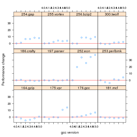
Figure 1. Percentage change in SPEC number (relative to version 4.0.4) for 12 programs compiled using 6 different versions of gcc (compiling to 64-bits with the O3 option).
Fitting a linear model requires at least two sets of [interval data]. The gcc version numbers are [ordinal values] and the following are two possible ways of mapping them to interval values:
-
there have been over 150 different released versions of gcc and a
particular version could be mapped to its place in this sequence. -
the date of release of a version can be mapped to the number of
days since the first release.
If version releases are organized around new functionality added then it makes sense to use version sequence number. If the performance of a new optimization was proportional to the amount of effort (e.g., man days) that went into its implementation then it would make sense to use days between releases.
The versions tested by Makarow were each from a different secondary release within a given primary version line and at roughly yearly intervals (two years separated the first pair and one month another pair).
There have been approximately 25 secondary releases in the 25 year project and using a release version sequence number starting at 20 seems like a reasonable choice.
Internally a compiler optimizer performs many different kinds of optimizations (gcc has over 160 different options for controlling machine independent optimization behavior). While the implementation of a new optimization is a gradual process involving many days of work, from the external user perspective it either exists and does its job when a given optimization level is supported or it does not exist.
What is the shape of the performance/release-version relationship? In the first few years of a compilers development it is to be expected that all the known major (i.e., big impact) optimization will be implemented and thereafter newly added optimizations have a progressively smaller impact on overall performance. Given gcc’s maturity it looks reasonable to assume that new releases contain a few additional improvement that have an incremental impact, i.e., the performance/release-version relationship is assumed to be linear (no other relationship springs out of a plot of the data).
A mixed-effects model can be created by calling the R function lme from the package nlme. The only difference between the following call to lme and a call to lm is the third argument specifying the random component.
t.lme=lme(value ~ variable, data=lme.O2, random = ~ 1 | Name) |
The argument random = ~ 1 | Name specifies that the random component effects the mean value of the result (when building a model this translates to an effect on the value of the intercept of the fitted equation) and that Name (of the program) is the grouped variable.
To specify that the random effect applies to the slope of the equation rather than its intercept the call is as follows:
t.lme=lme(value ~ variable, data=lme.O2, random = ~ variable -1 | Name) |
To specify that both the slope and the intercept are effected the -1 is omitted (for this gcc data the calculation fails to converge when both can be effected).
Since the measurements are about different versions of gcc it is to be expected that the data format has a separate column for each version of gcc (the format that would be used to pass data lm) as follows:
Name v3.2.3 v3.3.6 v3.4.6 v4.0.4 v4.1.2 v4.2.4 v4.3.1 v4.4.0 v4.5.0 1 164.gzip 933 932 957 922 933 939 917 969 955 2 175.vpr 562 561 577 576 586 585 576 589 588 3 176.gcc 1087 1084 1159 1135 1133 1102 1146 1189 1211 |
The relationship between the three variables in the call to lme is more complicated and the data needs to be reorganize so that one column contains all of the values, one the gcc version numbers and another column the program names. The function melt from package reshape2 can be used to restructure the data to look like:
Name variable value 11 256.bzip2 v3.2.3 0.000000 12 300.twolf v3.2.3 0.000000 13 SPECint2000 v3.2.3 0.000000 14 164.gzip v3.3.6 -0.107181 15 175.vpr v3.3.6 -0.177936 16 176.gcc v3.3.6 -0.275989 17 181.mcf v3.3.6 0.148810 |
Comparing O2 and O3 option performance
When comparing two samples the [Wilcoxon signed-rank test] and the [Mann-Whitney U test] spring to mind. However, some of the expected characteristics of the data violate some of the properties that these tests assume hold (e.g., every release include new/updated optimizations which is likely to result in the performance of each release having a different mean and variance).
The difference in performance between the two optimization levels could be treated as a set of values that could be modelled using the same techniques applied above. If the resulting model have a line than ran parallel with the x-axis and was within the appropriate confidence bounds we could claim that there was no measurable difference between the two options.
Results
The following is the output produced by summary for a mixed-effect model, with the random variation assumed to effect the value of intercept, created from the SPEC numbers for the integer programs compiled for 64-bit code at optimization level O2:
Linear mixed-effects model fit by REML
 Data: lme.O2
       AIC      BIC    logLik
  453.4221 462.4161 -222.7111

Random effects:
 Formula: ~1 | Name
        (Intercept) Residual
StdDev:    7.075923 4.358671

Fixed effects: value ~ variable
                 Value Std.Error DF   t-value p-value
(Intercept) -29.746927  7.375398 59 -4.033264   2e-04
variable      1.412632  0.300777 59  4.696612   0e+00
 Correlation:
         (Intr)
variable -0.958

Standardized Within-Group Residuals:
        Min          Q1         Med          Q3         Max
-4.68930170 -0.45549280 -0.03469526  0.31439727  2.45898648

Number of Observations: 72
Number of Groups: 12
|
and the following summary output is from a linear model built from an average of the data used above.
Call:
lm(formula = value ~ variable, data = lmO2)

Residuals:
      13       26       39       52       65       78
 0.16961 -0.32719  0.47820 -0.47819 -0.01751  0.17508

Coefficients:
             Estimate Std. Error t value Pr(>|t|)
(Intercept) -28.29676    2.22483  -12.72 0.000220 ***
variable      1.33939    0.09442   14.19 0.000143 ***
---
Signif. codes:  0 ‘***’ 0.001 ‘**’ 0.01 ‘*’ 0.05 ‘.’ 0.1 ‘ ’ 1

Residual standard error: 0.395 on 4 degrees of freedom
Multiple R-squared: 0.9805,     Adjusted R-squared: 0.9756
F-statistic: 201.2 on 1 and 4 DF,  p-value: 0.0001434
|
The biggest difference is that the fitted values for the Intercept and slope (the column name, variable, gives this value) have a standard error that is 3+ times greater for the mixed-effects model compared to the linear model based on using average values (a similar result is obtained if the mixed-effects random variation is assumed to effect the slope and the calculation fails to converge if the variation is on both intercept and slope). One consequence of building a linear model based on averaged values is that some of the variations present in the data are smoothed out. The mixed-effects model is more accurate in that it takes all variations present in the data into account.
For integer programs compiled for 32-bits there is much less difference between the mixed-effects models and linear models than is seen for 64-bit code.
-
For SPEC performance the created models show:
-
for the integer programs a rate of increase of around 0.6% (sd
0.2) per release forO2andO3options on 32-bit code
and an increase of 1.4% (sd 0.3) for 64-bit code, -
for floating-point, C programs only, a rate of increase per
release of 12% (sd 5) at 32-bits and 1.4% (sd 0.7) at 64-bits, with
very little difference between theO2andO3options.
-
for the integer programs a rate of increase of around 0.6% (sd
-
For size of generated code the created models show:
-
for integer programs 32-bit code built using
O2size is
decreasing at the rate of 0.6% (sd 0.1) per release, while for both
64-bit code andO3the size is increasing at between 0.7% (sd
0.2) and 2.5% (sd 0.4) per release, -
for floating-point, C programs only, 32-bit code built using
O2had an unacceptable p-value, while for both 64-bit code
andO3the size is increasing at between 1.6% (sd 0.3) and
9.3 (sd 1.1) per release.
-
for integer programs 32-bit code built using
Comparing O2 and O3 option performance
The intercept and slope values for the models built for the SPEC integer performance difference had p-values way too large to be of interest (a ballpark estimate of the values would suggest very little performance difference between the two options).
The program size change models showed O3 increasing, relative to O2, at 1.4% to 1.7% per release.
Discussion
The average rate of increase in SPEC number is very low and does not appear to be worth bothering about, possible reasons for this include:
-
a lot of effort has already been invested in making sure that gcc
performs well on the SPEC programs and the optimizations now being
added to gcc are aimed at programs having other kinds of
characteristics, -
gcc is a mature compiler that has implemented all of the worthwhile
optimizations and there are no more major improvements left to be
made, -
measurements based on just setting the
O2orO3
options might not provide a reliable guide to gcc optimization
performance. The command
gcc -c -Q -O2 --help=optimizers
shows that for gcc version 4.5.0 theO2option enables 91 of
the possible 174 optimization options and theO3option
enables 7 more. Performing some optimizations together sometimes
results in poorer quality code than if a subset of those
optimizations had been applied (genetic programming is being
researched as one technique for selecting the best optimizations
options to use for a given program and up to 13% improvements have
been obtained over gcc’s -O options <book Bashkansky_07>). The
percentage performance change figure above shows
that for some programs performance decreases on some releases.Whole program optimization is a major optimization area that has been addressed in recent versions of gcc, this optimizations is not enabled by the
Ooptions.
The percentage differences in SPEC integer performance between the O2 and O3 options were very small, but varied too much to be able to build a reliable linear model from the values.
For SPEC program code size there is a significant different between the O2 and O3 options. This is probably explained by function inlining being one of the seven additional optimization enabled by O3 (inlining multiple calls to the same function often increases code size <book inlining> and changes to the inlining optimization over releases could result in more functions being inlined).
Conclusion
Either the optimizations added to gcc between 2003 and 2010 have not made any significant difference to the performance of the generated code or the established method of measuring gcc optimization performance (i.e., the SPEC benchmarks and the O2 or O3 compiler options) is no longer a reliable indicator.
Compiler benchmarking for the 21st century
I would like to propose a new way of measuring the quality of a compiler’s code generator: The highest quality compiler is one that generates identical code for all programs that produce the same output, e.g., a compiler might spot programs that calculate pi and always generate code that uses the most rapidly converging method known. This is a very different approach to the traditional methods based on using (mostly) execution time or size (usually code but sometimes data) as a measure of quality.
Why is a new measurement method needed, and why choose this one? It is relatively easy for compiler vendors to tune their products to the commonly used benchmark and they seem to have lost their role as drivers for new optimization techniques. Different developers have different writing habits and companies should not have to waste time and money changing developer habits just to get the best quality code out of a compiler; compilers should handle differences in developer coding habits and not let it affect the quality of generated code. There are major savings to be had by optimizing the effect that developers are trying to achieve rather than what they have actually written (these days new optimizations targeting at what developers have written show very low percentage improvements).
Deducing that a function calculates pi requires a level of sophistication in whole program analysis that is unlikely to be available in production compilers for some years to come (ok, detecting 4*atan(1.0) is possible today). What is needed is a collection of compilable files containing source code that aims to achieve an outcome in lots of different ways. To get the ball rolling the “3n times 2” problem is presented as the first of this new breed of benchmarks.
The “3n times 2” problem is a variant on the 3n+1 problem that has been tweaked to create more optimization opportunities. One implementation of the “3n times 2” problem is:
if (is_odd(n)) n = 3*n+1; else n = 2*n; // this is n = n / 2; in the 3n+1 problem |
There are lots of ways of writing code that has the same effect, some of the statements I have seen for calculating n=3*n+1 include: n = n + n + n + 1, n = (n << 1) + n + 1 and n *= 3; n++, while some of the ways of checking if n is odd include: n & 1, (n / 2)*2 != n and n % 2.
I have created a list of different ways in which 3*n+1 might be calculated and is_odd(n) might be tested and written a script to generate a function containing all possible permutations (to reduce the number of combinations no variants were created for the least interesting case of n=2*n, which was always generated in this form). The following is a snippet of the generated code (download everything):
if (n & 1) n=(n << 2) - n +1; else n*=2; if (n & 1) n=3*n+1; else n*=2; if (n & 1) n += 2*n +1; else n*=2; if ((n / 2)*2 != n) { t=(n << 1); n=t+n+1; } else n*=2; if ((n / 2)*2 != n) { n*=3; n++; } else n*=2; |
Benchmarks need a means of summarizing the results and here I make a stab at doing that for gcc 4.6.1 and llvm 2.9, when executed using the -O3 option (output here and here). Both compilers generated a total of four different sequences for the 27 'different' statements (I'm not sure what to do about the inline function tests and have ignored them here) with none of the sequences being shared between compilers. The following lists the number of occurrences of each sequence, e.g., gcc generated one sequence 16 times, another 8 times and so on:
gcc    16   8   2   1
llvm   12   6   6   3
How might we turn these counts into a single number that enables compiler performance to be compared? One possibility is to award 1 point for each of the most common sequence, 1/2 point for each of the second most common, 1/4 for the third and so on. Using this scheme, gcc gets 20.625, and llvm gets 16.875. So gcc has greater consistency (I am loathed to use the much overused phrase higher quality).
Now for a closer look at the code generated.
Both compilers always generated code to test the least significant bit for the conditional expressions n & 1 and n % 2. For the test (n / 2)*2 != n gcc generated the not very clever right-shift/left-shift/compare while llvm and'ed out the bottom bit and then compared; so both compilers failed to handle what is a surprisingly common check for a number being odd.
The optimal code for n=3*n+1 on a modern x86 processor is (lots of register combinations are possible, let's assume rdx contains n) leal 1(%rdx,%rdx,2), %edx and this is what both compilers generated a lot of the time. This locally optimal code is not always generated because:
- gcc fails to detect that
(n << 2)-n+1is equivalent to(n << 1)+n+1and generates the sequenceleal 0(,%rax,4), %edx ; subl %eax, %edx ; addl $1, %edx(I pointed this out to a gcc maintainer sometime ago, and he suggested reporting it as a bug). This 'bug' occurs three times in total. - For some forms of the calculation llvm generates globally better code by taking the else arm into consideration. For instance, when the calculation is written as
n += (n << 1) +1llvm deduces that(n << 1)and the2*nin theelseare equivalent, evaluates this value into a register before performing the conditional test thus removing the need for an unconditional jump around the 'else' code:leal (%rax,%rax), %ecx testb $1, %al je .LBB0_8 # BB#7: orl $1, %ecx # deduced ecx is even, arithmetic unit not needed! addl %eax, %ecx .LBB0_8:
This more efficient sequence occurs nine times in total.
The most optimal sequence was generated by gcc:
testb $1, %dl leal (%rdx,%rdx), %eax je .L6 leal 1(%rdx,%rdx,2), %eax .L6: |
with llvm and pre 4.6 versions of gcc generating the more traditional form (above, gcc 4.6.1 assumes that the 'then' arm is the most likely to be executed and trades off a leal against a very slow jmp):
testb $1, %al je .LBB0_5 # BB#4: leal 1(%rax,%rax,2), %eax jmp .LBB0_6 .LBB0_5: addl %eax, %eax .LBB0_6: |
There is still room for improvement, perhaps by using the conditional move instruction (which gcc actually generates within the not-very-clever code sequence for (n / 2)*2 != n) or by using the fact that eax already holds 2*n (the potential saving would come through a reduction in complexity of the internal resources needed to execute the instruction).
llvm insists on storing the calculated value back into n at the end of every statement. I'm not sure if this is a bug or a feature designed to make runtime debugging easier (if so it ought to be switched off by default).
Missed optimization opportunities (not intended to be part of this benchmark and if encountered would require a restructuring of the test source) include noticing that if  is odd then
  is always even, creating the opportunity to perform the following multiply by 2 without an if test.
Perhaps one day, compilers will figure out when a program is calculating pi and generate code that uses the best known algorithm. In the meantime, I am interested in hearing suggestions for additional different-algorithm-same-code benchmarks.
Program optimization given 1,000 datasets
A recent paper reminded me of a consequence of widespread availability of multi-processor systems I had failed to mention in a previous post on compiler writing in the next decade. The wide spread availability of systems containing large numbers of processors opens up opportunities for both end users of compilers and compiler writers.
Some compiler optimizations involve making decisions about what parts of a program will be executed more frequently than other parts; usually speeding up the frequently executed at the expense of slowing down the less frequently executed. The flow of control through a program is often effected by the input it has been given.
Traditionally optimization tuning has been done by feeding a small number of input datasets into a small number of programs, with the lazy using only the SPEC benchmarks and the more conscientious (or perhaps driven by one very important customer) using a few more acquired over time. A few years ago the iterative compiler tuning community started to address this lack of input benchmark datasets by creating 20 datasets for each of their benchmark programs.
Twenty datasets was certainly a step up from a few. Now one group (Evaluating Iterative Optimization Across 1000 Data Sets; written by a team of six people) has used 1,000 different input data sets to evaluate the runtime performance of a program; in fact they test 32 different programs each having their own 1,000 data sets. Oh, one fact they forgot to mention in the abstract was that each of these 32 programs was compiled with 300 different combinations of compiler options before being fed the 1,000 datasets (another post talks about the problem of selecting which optimizations to perform and the order in which to perform them); so each program is executed 300,000 times.
Standing back from this one could ask why optimizers have to be ‘pre-tuned’ using fixed datasets and programs. For any program the best optimization results are obtained by profiling it processing large amounts of real life data and then feeding this profile data back to a recompilation of the original source. The problem with this form of optimization is that most users are not willing to invest the time and effort needed to collect the profile data.
Some people might ask if 1,000 datasets is too many, I would ask if it is enough. Optimization often involves trade-offs and benchmark datasets need to provide enough information to compiler writers that they can reliably tune their products. The authors of the paper are still analyzing their data and I imagine that reducing redundancy in their dataset is one area they are looking at. One topic not covered in their first paper, which I hope they plan to address, is how program power consumption varies across the different datasets.
Where next with the large multi-processor systems compiler writers now have available to them? Well, 32 programs is not really enough to claim reasonable coverage of all program characteristics that compilers are likely to encounter. A benchmark containing 1,000 different programs is the obvious next step. One major hurdle, apart from the people time involved, is finding 1,000 programs that have usable datasets associated with them.
Recent Comments