Archive
Ecosystems chapter of “evidence-based software engineering” reworked
The Ecosystems chapter of my evidence-based software engineering book has been reworked (I have given up on the idea that this second pass is also where the polishing happens; polishing still needs to happen, and there might be more material migration between chapters); download here.
I have been reading books on biological ecosystems, and a few on social ecosystems. These contain lots of interesting ideas, but the problem is, software ecosystems are just very different, e.g., replication costs are effectively zero, source code does not replicate itself (and is not self-evolving; evolution happens because people change it), and resources are exchanged rather than flowing (e.g., people make deals, they don’t get eaten for lunch). Lots of caution is needed when applying ecosystem related theories from biology, the underlying assumptions probably don’t hold.
There is a surprising amount of discussion on the computing world as it was many decades ago. This is because ecosystem evolution is path dependent; understanding where we are today requires knowing something about what things were like in the past. Computer memory capacity used to be a big thing (because it was often measured in kilobytes); memory does not get much publicity because the major cpu vendor (Intel) spends a small fortune on telling people that the processor is the most important component inside a computer.
There are a huge variety of software ecosystems, but you would not know this after reading the ecosystems chapter. This is because the work of most researchers has been focused on what used to be called the desktop market, which over the last few years the focus has been shifting to mobile. There is not much software engineering research focusing on embedded systems (a vast market), or supercomputers (a small market, with lots of money), or mainframes (yes, this market is still going strong). As the author of an evidence-based book, I have to go where the data takes me; no data, then I don’t have anything to say.
Empirical research (as it’s known in academia) needs data, and the ‘easy’ to get data is what most researchers use. For instance, researchers analyzing invention and innovation invariably use data on patents granted, because this data is readily available (plus everybody else uses it). For empirical research on software ecosystems, the readily available data are package repositories and the Google/Apple Apps stores (which is what everybody uses).
The major software ecosystems barely mentioned by researchers are the customer ecosystem (the people who pay for everything), the vendors (the companies in the software business) and the developer ecosystem (the people who do the work).
Next, the Projects chapter.
Compiler validation used to be a big thing
Compiler validation used to be a big thing; a NIST quarterly validated products list could run to nearly 150 pages, and approaching 1,000 products (not all were compilers).
Why did compiler validation stop being a thing?
Running a compiler validation service (NIST was also involved with POSIX, graphics, and computer security protocols validation) costs money. If there are enough people willing to pay (NIST charged for the validation service), the service pays for itself.
The 1990s was a period of consolidation, lots of computer manufacturers went out of business and Micro Focus grew to dominate the Cobol compiler business. The number of companies willing to pay for validation fell below the number needed to maintain the service; the service was terminated in 1998.
The source code of the Cobol, Fortran and SQL + others tests that vendors had to pass (to appear for 12 months in the validated products list) is still available; the C validation suite costs money. But passing these tests, then paying NIST’s fee for somebody to turn up and watch the compiler pass the tests, no longer gets your product’s name in lights (or on the validated products list).
At the time, those involved lamented the demise of compiler validation. However, compiler validation was only needed because many vendors failed to implement parts of the language standard, or implemented them differently. In many ways, reducing the number of vendors is a more effective means of ensuring consistent compiler behavior. Compiler monoculture may spell doom for those in the compiler business (and language standards), but is desirable from the developers’ perspective.
How do we know whether today’s compilers implement the requirements contained in the corresponding ISO language standard? You could argue that this is a pointless question, i.e., gcc and llvm are the language standard; but let’s pretend this is not the case.
Fuzzing is good for testing code generation. Checking language semantics still requires expert human effort, and lots of it. People have to extract the requirements contained in the language specification, and write code that checks whether the required behavior is implemented. As far as I know, there are only commercial groups doing this, i.e., nothing in the open source world; pointers welcome.
Converting lines in an svg image to csv
During a search for data on programming language usage I discovered Stack Overflow Trends, showing an interesting plot of language tags appearing on Stack Overflow questions (see below). Where was the csv file for these numbers? Somebody had asked this question last year, but there were no answers.

The graphic is in svg format; has anybody written an svg to csv conversion tool? I could only find conversion tools for specialist uses, e.g., geographical data processing. The svg file format is all xml, and using a text editor I could see the numbers I was after. How hard could it be (it had to be easier than a png heatmap)?
Extracting the x/y coordinates of the line segments for each language turned out to be straight forward (after some trial and error). The svg generation process made matching language to line trivial; the language name was included as an xml attribute.
Programmatically extracting the x/y axis information exhausted my patience, and I hard coded the numbers (code+data). The process involves walking an xml structure and R’s list processing, two pet hates of mine (the data is for a book that uses R, so I try to do everything data related in R).
I used R’s xml2 package to read the svg files. Perhaps if my mind had a better fit to xml and R lists, I would have been able to do everything using just the functions in this package. My aim was always to get far enough down to convert the subtree to a data frame.
Extracting data from graphs represented in svg files is so easy (says he). Where is the wonderful conversion tool that my search failed to locate? Pointers welcome.
My book’s pdf generation workflow
The process used to generate the pdf of my evidence-based software engineering book has been on my list of things to blog about, for ever. An email arrived this afternoon, asking how I produced various effects using Asciidoc; this post probably contains rather more than N. Psaris wanted to know.
It’s very easy to get sucked into fiddling around with page layout and different effects. So, unless I am about to make a release of a draft, I only generate a pdf once, at the end of each month.
At the end of the month the text is spell checked using aspell, and then grammar checked using Language tool. I have an awk script that checks the text for mistakes I have made in the past; this rarely matches, i.e., I seem to be forever making different mistakes.
The sequencing of tools is: R (Sweave) -> Asciidoc -> docbook -> LaTeX -> pdf; assorted scripts fiddle with the text between outputs and inputs. The scripts and files mention below are available for download.
R generates pdf files (via calls to the Sweave function, I have never gotten around to investigating Knitr; the pdfs are cropped using scripts/pdfcrop.sh) and the ascii package is used to produce a few tables with Asciidoc markup.
Asciidoc is the markup language used for writing the text. A few years after I started writing the book, Stuart Rackham, the creator of Asciidoc, decided to move on from working and supporting it. Unfortunately nobody stepped forward to take over the project; not a problem, Asciidoc just works (somebody did step forward to reimplement the functionality in Ruby; Asciidoctor has an active community, but there is no incentive for me to change). In my case, the output from Asciidoc is xml (it supports a variety of formats).
Docbook appears in the sequence because Asciidoc uses it to produce LaTeX. Docbook takes xml as input, and generates LaTeX as output. Back in the day, Docbook was hailed as the solution to all our publishing needs, and wonderful tools were going to be created to enable people to produce great looking documents.
LaTeX is the obvious tool for anybody wanting to produce lovely looking books and articles; tex/ESEUR.tex is the top-level LaTeX, which includes the generated text. Yes, LaTeX is a markup language, and I could have written the text using it. As a language I find LaTeX too low level. My requirements are not complicated, and I find it easier to write using a markup language like Asciidoc.
The input to Asciidoc and LuaTeX (used to generate pdf from LaTeX) is preprocessed by scripts (written using sed and awk; see scripts/mkpdf). These scripts implement functionality that Asciidoc does not support (or at least I could see how to do it without modifying the Python source). Scripts are a simple way of providing the extra functionality, that does not require me to remember details about the internals of Asciidoc. If Asciidoc was being actively maintained, I would probably have worked to get some of the functionality integrated into a future release.
There are a few techniques for keeping text processing scripts simple. For instance, the cost of a pass over text is tiny, there is little to be gained by trying to do everything in one pass; handling the possibility that markup spans multiple lines can be complicated, a simple solution is to join consecutive lines together if there is a possibility that markup spans these lines (i.e., the actual matching and conversion no longer has to worry about line breaks).
Many simple features are implemented by a script modifying Asciidoc text to include some ‘magic’ sequence of characters, which is subsequently matched and converted in the generated LaTeX, e.g., special characters, and hyperlinks in the pdf.
A more complicated example handles my desire to specify that a figure appear in the margin; the LaTeX sidenotes package supports figures in margins, but Asciidoc has no way of specifying this behavior. The solution was to add the word “Margin”, to the appropriate figure caption option (in the original Asciidoc text, e.g., [caption="Margin ", label=CSD-95-887]), and have a script modify the LaTeX generated by docbook so that figures containing “Margin” in the caption invoked the appropriate macro from the sidenotes package.
There are still formatting issues waiting to be solved. For instance, some tables are narrow enough to fit in the margin, but I have not found a way of embedding this information in the table information that survives through to the generated LaTeX.
My long time pet hate is the formatting used by R’s plot function for exponentiated values as axis labels. My target audience are likely to be casual users of R, so I am sticking with basic plotting (i.e., no calls to ggplot). I do wish the core R team would integrate the code from the magicaxis package, to bring the printing of axis values into the era of laser printers and bit-mapped displays.
Ideas and suggestions welcome.
Growth and survival of gcc options and processor support
Like any actively maintained software, compilers get more complicated over time. Languages are still evolving, and options are added to control the support for features. New code optimizations are added, which don’t always work perfectly, and options are added to enable/disable them. New ways of combining object code and libraries are invented, and new options are added to allow the desired combination to be selected.
The web pages summarizing the options for gcc, for the 96 versions between 2.95.2 and 9.1 have a consistent format; which means they are easily scrapped. The following plot shows the number of options relating to various components of the compiler, for these versions (code+data):
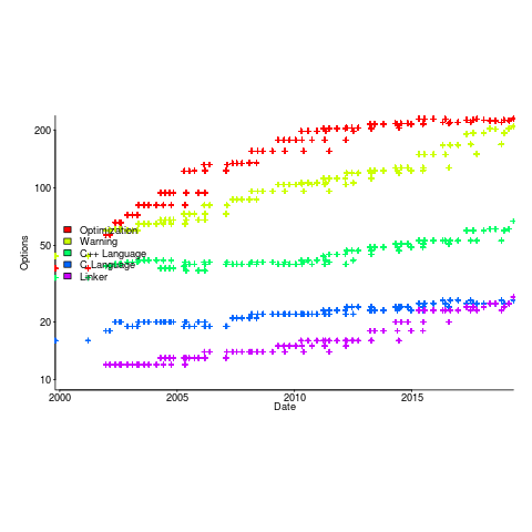
The total number of options grew from 632 to 2,477. The number of new optimizations, or at least the options supporting them, appears to be leveling off, but the number of new warnings continues to increase (ah, the good ol’ days, when -Wall covered everything).
The last phase of a compiler is code generation, and production compilers are generally structured to enable new processors to be supported by plugging in an appropriate code generator; since version 2.95.2, gcc has supported 80 code generators.
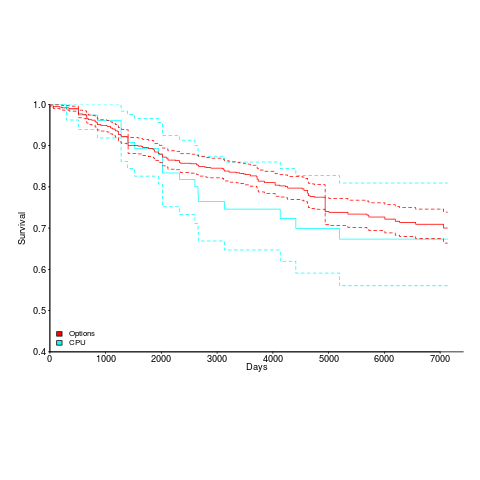
What can be added can be removed. The plot below shows the survival curve of gcc support for processors (80 supported cpus, with support for 20 removed up to release 9.1), and non-processor specific options (there have been 1,091 such options, with 214 removed up to release 9.1); the dotted lines are 95% confidence internals.
Recent Comments