Archive
McCabe’s cyclomatic complexity and accounting fraud
The paper in which McCabe proposed what has become known as McCabe’s cyclomatic complexity did not contain any references to source code measurements, it was a pure ego and bluster paper.
Fast forward 10 years and cyclomatic complexity, complexity metric, McCabe’s complexity…permutations of the three words+metrics… has become one of the two major magical omens of code quality/safety/reliability (Halstead’s is the other).
It’s not hard to show that McCabe’s complexity is a rather weak measure of program complexity (it’s about as useful as counting lines of code).
Just as it is possible to reduce the number of lines of code in a function (by putting all the code on one line), it’s possible to restructure existing code to reduce the value of McCabe’s complexity (which is measured for individual functions).
The value of McCabe’s complexity for the following function is 5 16, i.e., and there are 16 possible paths through the function:
int main(void) { if (W) a(); else b(); if (X) c(); else d(); if (Y) e(); else f(); if (Z) g(); else h(); } |
each if…else contains two paths and there are four in series, giving  paths.
Restructuring the code, as below, removes the multiplication of paths caused by the sequence of if…else:
void a_b(void) {if (W) a(); else b();} void c_d(void) {if (X) c(); else d();} void e_f(void) {if (Y) e(); else f();} void g_h(void) {if (Z) g(); else h();} int main(void) { a_b(); c_d(); e_f(); g_h(); } |
reducing main‘s McCabe complexity to 1 and the four new functions each have a McCabe complexity of two.
Where has the ‘missing’ complexity gone? It now ‘exists’ in the relationship between the functions, a relationship that is not included in the McCabe complexity calculation.
The number of paths that can be traversed, by a call to main, has not changed (but the McCabe method for counting them now produces a different answer)
Various recommended practice documents suggest McCabe’s complexity as one of the metrics to consider (but don’t suggest any upper limit), while others go as far as to claim that it’s bad practice for functions to have a McCabe’s complexity above some value (e.g., 10) or that “Cyclomatic complexity may be considered a broad measure of soundness and confidence for a program“.
Consultants in the code quality/safety/security business need something to complain about, that is not too hard or expensive for the client to fix.
If a consultant suggested that you reduced the number of lines in a function by joining existing lines, to bring the count under some recommended limit, would you take them seriously?
What about, if a consultant highlighted a function that had an allegedly high McCabe’s complexity? Should what they say be taken seriously, or are they essentially encouraging developers to commit the software equivalent of accounting fraud?
Top, must-read paper on software fault analysis
What is the top, must read, paper on software fault analysis?
Software Reliability: Repetitive Run Experimentation and Modeling by Phyllis Nagel and James Skrivan is my choice (it’s actually a report, rather than a paper). Not only is this report full of interesting ideas and data, but it has multiple replications. Replication of experiments in software engineering is very rare; this work was replicated by the original authors, plus Scholz, and then replicated by Janet Dunham and John Pierce, and then again by Dunham and Lauterbach!
I suspect that most readers have never heard of this work, or of Phyllis Nagel or James Skrivan (I hadn’t until I read the report). Being published is rarely enough for work to become well-known, the authors need to proactively advertise the work. Nagel, Dunham & co worked in industry and so did not have any students to promote their work and did not spend time on the academic seminar circuit. Given enough effort it’s possible for even minor work to become widely known.
The study run by Nagel and Skrivan first had three experienced developers independently implement the same specification. Each of these three implementations was then tested, multiple times. The iteration sequence was: 1) run program until fault experienced, 2) fix fault, 3) if less than five faults experienced, goto step (1). The measurements recorded were fault identity and the number of inputs processed before the fault was experienced.
This process was repeated 50 times, always starting with the original (uncorrected) implementation; the replications varied this, along with the number of inputs used.
For a fault to be experienced, there has to be a mistake in the code and the ‘right’ input values have to be processed.
How many input values need to be processed, on average, before a particular fault is experienced? Does the average number of inputs values needed for a fault experience vary between faults, and if so by how much?
The plot below (code+data) shows the numbers of inputs processed, by one of the implementations, before individual faults were experienced, over 50 runs (sorted by number of inputs):
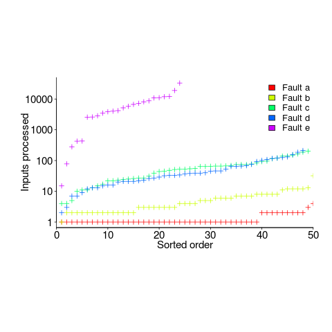
Different faults have different probabilities of being experienced, with fault a being experienced on almost any input and fault e occurring much less frequently (a pattern seen in the replications). There is an order of magnitude variation in the number of inputs processed before particular faults are experienced (this pattern is seen in the replications).
Faults were fixed as soon as they were experienced, so the technique for estimating the total number of distinct faults, discussed in a previous post, cannot be used.
A plot of number of faults found against number of inputs processed is another possibility. More on that another time.
Suggestions for top, must read, paper on software faults, welcome (be warned, I think that most published fault research is a waste of time).
Estimating the number of distinct faults in a program
In an earlier post I gave two reasons why most fault prediction research is a waste of time: 1) it ignores the usage (e.g., more heavily used software is likely to have more reported faults than rarely used software), and 2) the data in public bug repositories contains lots of noise (i.e., lots of cleaning needs to be done before any reliable analysis can done).
Around a year ago I found out about a third reason why most estimates of number of faults remaining are nonsense; not enough signal in the data. Date/time of first discovery of a distinct fault does not contain enough information to distinguish between possible exponential order models (technical details; practically all models are derived from the exponential family of probability distributions); controlling for usage and cleaning the data is not enough. Having spent a lot of time, over the years, collecting exactly this kind of information, I was very annoyed.
The information required, to have any chance of making a reliable prediction about the likely total number of distinct faults, is a count of all fault experiences, i.e., multiple instances of the same fault need to be recorded.
The correct techniques to use are based on work that dates back to Turing’s work breaking the Enigma codes; people have probably heard of Good-Turing smoothing, but the slightly later work of Good and Toulmin is applicable here. The person whose name appears on nearly all the major (and many minor) papers on population estimation theory (in ecology) is Anne Chao.
The Chao1 model (as it is generally known) is based on a count of the number of distinct faults that occur once and twice (the Chao2 model applies when presence/absence information is available from independent sites, e.g., individuals reporting problems during a code review). The estimated lower bound on the number of distinct items in a closed population is:

and its standard deviation is:
![S_{sd-est}={f_1}/{f_2}k sqrt{f_2(0.5/{k}+{f_1}/{f_2} [1+0.25 {f_1}/{f_2}])}](https://shape-of-code.com/wp-content/plugins/wpmathpub/phpmathpublisher/img/math_977.5_e69346120e72f31d04a47c9fcf64c4dd.png "S_{sd-est}={f_1}/{f_2}k sqrt{f_2(0.5/{k}+{f_1}/{f_2} [1+0.25 {f_1}/{f_2}])}")
where:  is the estimated number of distinct faults,
  the observed number of distinct faults,
  the total number of faults,
  the number of distinct faults that occurred once,
  the number of distinct faults that occurred twice,
  .
.
A later improved model, known as iChoa1, includes counts of distinct faults occurring three and four times.
Where can clean fault experience data, where the number of inputs have been controlled, be obtained? Fuzzing has become very popular during the last few years and many of the people doing this work have kept detailed data that is sometimes available for download (other times an email is required).
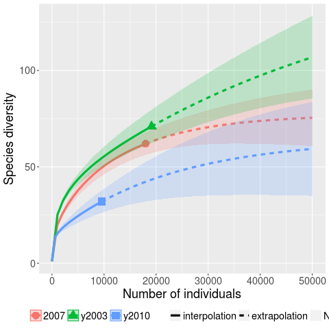
Kaminsky, Cecchetti and Eddington ran a very interesting fuzzing study, where they fuzzed three versions of Microsoft Office (plus various Open Source tools) and made their data available.
The faults of interest in this study were those that caused the program to crash. The plot below (code+data) shows the expected growth in the number of previously unseen faults in Microsoft Office 2003, 2007 and 2010, along with 95% confidence intervals; the x-axis is the number of faults experienced, the y-axis the number of distinct faults.
The take-away point: if you are analyzing reported faults, the information needed to build models is contained in the number of times each distinct fault occurred.
Historians of computing
Who are the historians of computing? The requirement I used for deciding who qualifies (for this post), is that the person has written multiple papers on the subject over a period that is much longer than their PhD thesis (several people have written a history of some aspect of computing PhDs, and then gone on to research other areas).
Maarten Bullynck. An academic who is a historian of mathematics and has become interested in software; use HAL to find his papers, e.g., What is an Operating System? A historical investigation (1954–1964).
Martin Campbell-Kelly. An academic who has spent his research career investigating computing history, primarily with a software orientation. Has written extensively on a wide variety of software topics. His book “From Airline Reservations to Sonic the Hedgehog: A History of the Software Industry” is still on my pile of books waiting to be read (but other historian cite it extensively). His thesis: “Foundations of computer programming in Britain, 1945-55″, can be freely downloadable from the British Library; registration required.
Paul E. Ceruzzi. An academic and museum curator; interested in aeronautics and computers. I found the one book of his that I have read, ok; others might like it more than me. Others cite him, and he wrote an interesting paper on Konrad Zuse (The Early Computers of Konrad Zuse, 1935 to 1945).
James W. Cortada. Ex-IBM (1974-2012) and now working at the Charles Babbage Institute. Written extensively on the history of computing. More of a hardware than software orientation. Written lots of detail oriented books and must have pole position for most extensive collection of material to cite (his end notes are very extensive). His “The Digital Flood: The Diffusion of Information Technology Across the U.S., Europe, and Asia” is likely to be the definitive work on the subject for some time to come. For me this book is spoiled by the author towing the company line in his analysis of the IBM antitrust trial; my analysis of the work Cortada cites reaches the opposite conclusion.
Nathan Ensmenger. An academic; more of a people person than hardware/software. His paper Letting the Computer Boys Take Over contains many interesting insights. His book The Computer Boys Take Over Computers, Programmers, and the Politics of Technical Expertise is a combination of topics that have been figured out, backed-up with references, and topics still being figured out (I wish he would not cite Datamation, a trade mag back in the day, so often).
Kenneth S. Flamm. An academic who has held senior roles in government. Writes from a industry evolution, government interests, economic perspective. The books: “Targeting the Computer: Government Support and International Competition” and “Creating the Computer: Government, Industry and High Technology” are packed with industry related economic data and covers all the major industrial countries.
Michael S. Mahoney. An academic who is sadly no longer with us. A historian of mathematics before becoming primarily involved with software history.
Jeffrey R. Yost. An academic. I have only read his book “Making IT Work: A history of the computer services industry”, which was really a collection of vignettes about people, companies and events; needs some analysis. Must try to track down some of his papers (which are not available via his web page :-(.
Who have I missed? This list is derived from papers/books I have encountered while working on a book, not an active search for historians. Suggestions welcome.
Updates
Completely forgot Kenneth S. Flamm, despite enjoying both his computer books.
Forgot Paul E. Ceruzzi because I was unimpressed by his “A History of Modern Computing”. Perhaps his other books are better.
Building a regression model is easy and informative
Running an experiment is very time-consuming. I am always surprised that people put so much effort into gathering the data and then spend so little effort analyzing it.
The Computer Language Benchmarks Game looks like a fun benchmark; it compares the performance of 27 languages using various toy benchmarks (they could not be said to be representative of real programs). And, yes, lots of boxplots and tables of numbers; great eye-candy, but what do they all mean?
The authors, like good experimentalists, make all their data available. So, what analysis should they have done?
A regression model is the obvious choice and the following three lines of R (four lines if you could the blank line) build one, providing lots of interesting performance information:
cl=read.csv("Computer-Language_u64q.csv.bz2", as.is=TRUE)

cl_mod=glm(log(cpu.s.) ~ name+lang, data=cl)
summary(cl_mod) |
The following is a cut down version of the output from the call to summary, which summarizes the model built by the call to glm.
                    Estimate Std. Error t value Pr(>|t|)
(Intercept)         1.299246   0.176825   7.348 2.28e-13 ***
namechameneosredux  0.499162   0.149960   3.329 0.000878 ***
namefannkuchredux   1.407449   0.111391  12.635  < 2e-16 ***
namefasta           0.002456   0.106468   0.023 0.981595
namemeteor         -2.083929   0.150525 -13.844  < 2e-16 ***

langclojure         1.209892   0.208456   5.804 6.79e-09 ***
langcsharpcore      0.524843   0.185627   2.827 0.004708 **
langdart            1.039288   0.248837   4.177 3.00e-05 ***
langgcc            -0.297268   0.187818  -1.583 0.113531
langocaml          -0.892398   0.232203  -3.843 0.000123 ***

    Null deviance: 29610  on 6283  degrees of freedom
Residual deviance: 22120  on 6238  degrees of freedom
What do all these numbers mean?
We start with glm's first argument, which is a specification of the regression model we are trying to fit: log(cpu.s.) ~ name+lang
cpu.s. is cpu time, name is the name of the program and lang is the language. I found these by looking at the column names in the data file. There are other columns in the data, but I am running in quick & simple mode. As a first stab, I though cpu time would depend on the program and language. Why take the log of the cpu time? Well, the model fitted using cpu time was very poor; the values range over several orders of magnitude and logarithms are a way of compressing this range (and the fitted model was much better).
The model fitted is:
 , or
, or 
Plugging in some numbers, to predict the cpu time used by say the program chameneosredux written in the language clojure, we get:  (values taken from the first column of numbers above).
This model assumes there is no interaction between program and language. In practice some languages might perform better/worse on some programs. Changing the first argument of glm to: log(cpu.s.) ~ name*lang, adds an interaction term, which does produce a better fitting model (but it's too complicated for a short blog post; another option is to build a mixed-model by using lmer from the lme4 package).
We can compare the relative cpu time used by different languages. The multiplication factor for clojure is  , while for
 ocaml it is  . So
. So clojure consumes 8.2 times as much cpu time as ocaml.
How accurate are these values, from the fitted regression model?
The second column of numbers in the summary output lists the estimated standard deviation of the values in the first column. So the clojure value is actually }") , i.e., between 2.2 and 4.9 (the multiplication by 1.96 is used to give a 95% confidence interval); the
, i.e., between 2.2 and 4.9 (the multiplication by 1.96 is used to give a 95% confidence interval); the ocaml values are }") , between 0.3 and 0.6.
, between 0.3 and 0.6.
The fourth column of numbers is the p-value for the fitted parameter. A value of lower than 0.05 is a common criteria, so there are question marks over the fit for the program fasta and language gcc. In fact many of the compiled languages have high p-values, perhaps they ran so fast that a large percentage of start-up/close-down time got included in their numbers. Something for the people running the benchmark to investigate.
Isn't it easy to get interesting numbers by building a regression model? It took me 10 minutes, ok I spend a lot of time fitting models. After spending many hours/days gathering data, spending a little more time learning to build simple regression models is well worth the effort.
Recent Comments