Archive
Working with an LLM maths assistant to model software processes
This post is a overview of the techniques I use when working with LLMs as a mathematics assistant to derive equations for the aggregate behavior of a collection of software processes. Much of the following could well apply to non-software processes, but my experience is software based.
Any analysis starts with one or more questions/problems and the environment within which any answer is likely to be applicable. Possible questions include:
- Expected number of lines of code, LOC, in the next release of a program,
- number of distinct statement sequences that can be written using

if-statements and
assignmentstatements, - fraction of a program’s functions/methods that have not been modified after fixing all reported faults.
Prompting an LLM with a software related question is likely to result in it giving a software related answer summarising statements made on blogs and perhaps findings from various research papers. These summaries may, or may not, contain the desired answer.
Obtaining a mathematical answer requires that a mathematical question be asked. The software question has to be reframed in mathematical terms. This requires some creativity, lateral thinking, and prior experience is very helpful.
For instance, for question 1, expected lines of code could be reframed as a recurrence relation, such as  , where:
  is the LOC in the
  ‘th release, and
  ,
,  are constants. An LLM can solve this to relation to give an equation for based on , , and
  (the size of the first release).
A more sophisticated set of recurrence relations could include the number of developers working on the project, along the probability distribution of the number of LOC they produce per day/week/month/release, and an equation for the expected time between releases.
Expressing question 2 in mathematical terms requires some lateral thinking. One possibility is to treat each line of code as a step on a 2-D lattice. An assignment statement occupying a line is one step down the page, while an if-statement occupies both a line and is (usually) indented to the right of the previous statement at the start, and indented to the left when it ends. Paths through a lattice are a well studied problem, with lots of existing mathematics for LLMs to have been trained on. This reframing of the question was good enough for me to be able to shepherd ChatGPT towards deriving an answer to the question. My pre-LLM research for answering a related question helped.

Creating a mathematical description of a question requires a lot of hard thinking (at least it does for me), and is an iterative process. If you are lucky, a good enough mapping to a starting formula is found, and the mathematics appears in textbooks, e.g., question 1. For other questions, lateral thinking may produce a mapping to a well researched area within some mathematical niche, e.g., question 2.
Creating a correct mathematical specification of the question is essential. Get this specification wrong, and any final equation will be the answer to a different question than the one intended. Mathematicians are used to describing problems in mathematical terms, while non-mathematicians (like me, and I suspect many readers) are likely to make mistakes and under/over specify the problem.
What can be done to check whether an LLM has interpreted the question in the way intended?
LLM chain-of-thought output provides the required feedback about how it interprets the question given. Some LLMs provide chain-of-thought output of their interpretation of the information contained in the prompt (e.g., Deepseek and Kimi), while others (e.g., until recently both ChatGPT and Grok; both have improved in the last few months) provide none, i.e., they are silent for a long time before giving an answer (which is can be useful for double-checking the output from other LLMs, but is otherwise of little use).
The following discussion is based on the process I used to obtain an answer to question 3.
The number of ways of placing some number of balls in some number of boxes is an established mathematical area of study that can be mapped to question 3. Functions are treated as empty boxes and fault reports as balls that are randomly placed in these boxes.
The initial mathematical question contains the minimum of constraints, and successive questions added constraints to better mimic the characteristics of source code and fault reports.
The following was my starting question:
$m$ identical boxes can each hold a maximum of $L$ balls, and there are $b$ identical balls, balls are uniformly at randomly placed in non-full boxes, where $L < m$ and $m*L > b$ and $b$ can have a similar size as $m$ What is the expected number of boxes that do not contain a ball |
The mathematics is enclosed in $ characters. LLMs support LaTeX input and output mathematics using LaTeX.
The first two lines specify the structure of the system. It’s important to specify that the balls are identical, otherwise the LLM has to decide whether they are, or are not, identical (non-identical has a very different solution).
The third line specifies the process behavior. The phrase “uniformly at randomly” is the mathematical way of saying “the behavior is random with all possibilities being equally likely”. When I first started using LLMs, this phrase is not something I used. However, “uniformly at randomly” often appeared in LLM output, so I switched to using it (LLMs having been trained on a lot more maths than me).
Lines four and five specify relationships between variables. Sometimes constraints such as these reduce the space of possibilities, and lead to a more concise answer. These constraints specify that a function will not contain more reported faults than it has lines of code (which is not always true), and that a program will not have more reported faults than lines of code.
The last line is the question I want answered (Kimi response).
In practice functions don’t all have the same size. Most functions are short, with fewer longer ones. The number of functions containing a given number of lines has (roughly) a power law distribution. Adding this information to the problem gives:
There are $m$ boxes, $B_n$, $1 <= n <= m$ where the
number of boxes that can hold $L$ balls, $1 <= L <= T$,
is proportional to $L^{-b}$,
and there are $F$ identical balls,
balls are uniformly at randomly placed in non-full boxes,
where the number of balls $F$ is much less than
the available places to hold them.
What is the expected number of boxes that do not contain a ball |
Boxes can now have different sizes, so they need to be labelled (i.e., $B_n$), with ball carrying capacity specified as a power law, i.e., $L^{-b}$.
The explicit constraints previously given are replaced by the general statement: “… the number of balls $F$ is much less than the available places to hold them.” This gives the LLM some flexibility about how to interpret the constraint.
LLMs make mistakes. I have seen them make a basic algebra mistake on one output line, followed by output that looks like penetrating insight (if a human had made it).
The chain-of-thought output reads like a derivation that a human would write (at least it does for Kimi, Deepseek, and recently GLM 5.1 from Z.ai). Checking the correctness of this derivation is necessary to gain confidence that the final answer is correct, or not.
This chain-of-thought often makes use a theorem or identity that is new to me. Kimi’s response to the updated prompt above made use of the polylogarithm function, which I had heard of, but knew nothing about.
When new to me maths is generated, Wikipedia is the first place I look. However, some Wikipedia maths articles appear to be written by mathematicians, who assume the reader already understands the topic, and simply summarise the relevant details; which is useless. Of course, one can always ask an LLM (a different one, so there is some cross-checking).
If the chain-of-thought looks correct, is the answer correct?
An LLM once give me an answer that was obviously wrong. It was an equation that could produce negative values, and in practice only positive values were possible. Each step of the chain-of-thought looked correct. It took me a while to spot that two disjoint assumptions in the LLM analysis combined to produce the incorrect answer.
I usually have an expectation of the behavior of any answer. Plotting the value of the equation given in an answer can show whether it follows the pattern of expected behavior.
Another way of gaining confidence in the answer is to give the prompt to multiple LLMs. Sometimes they all agree, and sometimes they disagree. The disagreement may be because the answer has been written in a slightly different form (e.g., summing a series from zero rather than one), or because the LLMs made slightly different assumptions. Comparing chain-of-thought will locate the points where assumptions diverge.
The third major iteration tried to address the observation that some functions are executed more often than others, and so are more likely to be involved in a fault report.
The specification was updated to include a preferential attachment component, with a box containing a ball having a higher probability of receiving a ball than one that did not contain a ball. The added text:
balls are randomly placed in non-full boxes with probability proportional to $L*(1+O)$ where $O$ is the number of ballscurrently in the box,
The equation in the answer was rather complicated (ChatGPT response). I have not checked this equation.
Most of the mathematically oriented questions/problems I have worked on have turned out to have uninteresting answers. Knowing this I can cross them off my list of things to think about. A few might lead to something interesting (e.g., fault prediction is starting to look like a waste of time), but need more work.
The answer checking process increases confidence that a particular answer is a solution to the question asked. It is possible that the specification of the question asked does not have a strong connection to reality.
My current first choice of LLMs for mathematical problems are Deepseek, Kimi, and recently GLM 5.1 (which has compute availability issues). This is primarily because they provide chain-of-thought output. In the last few months both ChatGPT and Grok have started providing more chain-of-thought output.
I usually start with one LLM to refine the question, and depending on progress later involve other LLMs to check and verify output.
Likelihood of encountering a given sequence of statements
How many lines of code have to be read to be likely to encounter every meaningful sequence of  statements (a non-meaningful sequence would be the three statements
 break;break;break;)?
First, it is necessary to work out the likelihood of encountering a given sequence of statements within lines of code.
If we just consider statements, then the following shows the percentage occurrence of the four kinds of C language statements (detailed usage information):
Statement % occurrence expression-stmt 60.3 selection-stmt 21.3 jump-stmt 15.0 iteration-stmt 3.4 |
The following analysis assumes that one statement occupies one line (I cannot locate data on percentage of statements spread over multiple lines).
An upper estimate can be obtained by treating this as an instance of the Coupon collector’s problem (which assumes that all items are equally likely), i.e., treating each sequence of statements as a coupon.
The average number of items that need to be processed before encountering all  distinct items is:
 =n*H_n") , where
, where  is the n-th harmonic number. When we are interested in at least one instance of every kind of C statement (i.e., the four listed above), we have:
 =8.33 right 9") .
.
There are  distinct sequences of three statements, but only
  meaningful sequences (when statements are not labelled, a
 jump-stmt can only appear at the end of a sequence). If we treat each of these 36 sequences as distinct, then =150.3 right 151") , 3-line sequences, or 453 LOC.
, 3-line sequences, or 453 LOC.
This approach both under- and over-estimates.
One or more statements may be part of different distinct sequences (causing the coupon approach to overestimate LOC). For instance, the following sequence of four statements:
expression-stmt selection-stmt expression-stmt expression-stmt |
contains two distinct sequences of three statements, i.e., the following two sequences:
expression-stmt selection-stmt selection-stmt expression-stmt expression-stmt expression-stmt |
There is a factor of 20-to-1 in percentage occurrence between the most/least common kind of statement. Does subdividing each kind of statement reduce this difference?
If expression-stmt, selection-stmt, and iteration-stmt are subdivided into their commonly occurring forms, we get the following percentages (where -other is the subdivision holding all cases whose occurrence is less than 1%, and the text to the right of sls- indicates the condition in an if-statement; data):
Statement % occurrence exs-func-call 22.3 exs-object=object 9.6 exs-object=func-call 6.0 exs-object=constant 4.2 exs-object_v++ 2.4 exs-other 15.7 sls-object 3.3 sls-object==object 1.9 sls-!object 1.6 sls-func-call 1.6 sls-expression 1.2 sls-other 11.7 jump-stmt 15.0 its-for 2.1 its-while 1.1 |
Function calls could be further broken down by number of arguments, but this would not have much impact because zero and one arguments are very common.
A more accurate model of the problem is needed.
A Markov chain approach handles both overlapping sequences, and statements having difference occurrence probabilities. For a sequence of length , the calculation involves an ") by matrix. For a sequence of three of the same kind of statement (chosen because ‘same kind’ of sequences are least likely to match, for a given length), the transition matrix is:
by matrix. For a sequence of three of the same kind of statement (chosen because ‘same kind’ of sequences are least likely to match, for a given length), the transition matrix is:
")
where  is the probability that statement
  will occur. The last row is the absorbing state. For the general case, see: Pattern Markov chains: Optimal Markov chain embedding through deterministic finite automata.
To calculate the probability that a sequence of the same kind of statement, of length , occurs within a sequence of statements, this transition matrix is multiplied  times (i.e., raised to the power ). The following code is an implementation in R (python script handling the general case):
seq_prob = function(N, s_len, Sk)
{
Sp=rep(Sk, s_len)
P=matrix(0, nrow = s_len+1, ncol = s_len+1) # Transition matrix
P[ , 1]=1-c(Sp, 1) # Probability of not occurring: first column
op=cbind(1:s_len, (1:s_len)+1) # diagonal for occurrence probabilities
P[op]=Sp           # assign occurrence probabilities
P[s_len+1, s_len+1]=1 # absorbing state

R=P # result value
for (n in 2:N)
   R=R %*% P # matrix multiply

return(R)
}

# Calculate probability for N equiprobable occurrences
# Result in last column of first row
N = 100
seq_len=3
sk=0.01
likelihood=seq_prob(N, seq_len, sk)[1, seq_len+1] |
If the occurrence likelihood of  (i.e., 1%), then the likelihood of encountering a sequence of three such statements in a sequence of 3 lines is
  (i.e., 0.0001%), while for a sequence of 100 lines it is
  .
.
The number of statements contained in a function varies. To calculate the likelihood of encountering a particular sequence of three statements in a program, or collection of programs, we need to find the likelihood over all function lengths, adjusting for the probability of encountering functions containing a given number of statements.
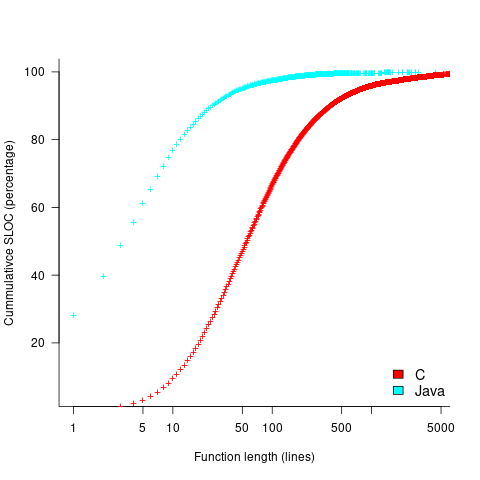
The plot below shows the cumulative percentage of code as function LOC increases (data from Landman, Serebrenik, Bouwers and Vinju; plot code):
Calculating the likelihood of encountering a given sequence length in a function containing a given number of LOC (ignoring local definitions and blank lines), and then adjusting for the probability of a function containing a given number of LOC, the likelihood of encountering a sequence containing 3-to-10 of the same kind of statement (whose likelihood of occurrence is 1%) is given by the following table (calculation code):
of
seq length   Occurrence likelihood
    3               2.3e-05
    4               2.2e-07
    5               2.1e-09
    6               2.0e-11
    7               2.0e-13
    8               1.9e-15
    9               1.8e-17
10 1.8e-19 |
These values can be used to calculate the likelihood of encountering this ‘1%’ statement sequence in a repo containing C functions. For instance, in 1 million functions the likelihood of one instance of a three ‘1%’ same-kind statement sequence is: ^{10^6} approx 1") . For a repo containing one billion functions of C, there is an 88% chance of encountering a sequence of five such statements.
. For a repo containing one billion functions of C, there is an 88% chance of encountering a sequence of five such statements.
The sequence occurrence likelihood for Java will be smaller because Java functions contain fewer LOC.
At the subdivision level of kind-of-statement that has been found to occur in 1% of all statements, sequences up to five long are likely to be encountered at least once in a billion functions, with sequences containing more common statements occurring at a greater rate.
Sequences of kind-of-statements whose occurrence rate is well below 1% are unlikely to be encountered.
This analysis has assumed that the likelihood of occurrence of each statement in a sequence is independent of the other statements in the sequence. For some kind-of-statement this is probably not true, but no data is available.
The pervasive use of common statement sequences enables LLMs to do a good job of predicting what comes next.
Transition probabilities when adjacent sequence items must be different
Generating a random sequence from a fixed set of items is a common requirement, e.g., given the items A, B and C we might generate the sequence BACABCCBABC. Often the randomness is tempered by requirements such as each item having each item appear a given number of times in a sequence of a given length, e.g., in a random sequence of 100 items A appears 20 times, B 40 times and C 40 times. If there are rules about what pairs of items may appear in the sequence (e.g., no identical items adjacent to each other), then sequence generation starts to get a bit complicated.
Let’s say we want our sequence to contain: A 6 times, B 12 times and C 12 times, and no same item pairs to appear (i.e., no AA, BB or CC). The obvious solution is to use a transition matrix containing the probability of generating the next item to be added to the end of the sequence based on knowing the item currently at the end of the sequence.
My thinking goes as follows:
- given A was last generated there is an equal probability of it being followed by B or C,
- given B was last generated there is a 6/(6+12) probability of it being followed by A and a 12/(6+12) probability of it being followed by C,
- given C was last generated there is a 6/(6+12) probability of it being followed by A and a 12/(6+12) probability of it being followed by B.
giving the following transition matrix (this row by row approach having the obvious generalization to more items):
                 Second item
               A      B       C
          A    0     .5      .5
First
item      B   .33     0      .67

C .33 .67 0 |
Having read Generating constrained randomized sequences: Item frequency matters by Robert M. French and Pierre Perruchet (from whom I take these examples and algorithm on which the R code is based), I now know this algorithm for generating transition matrices is wrong. Before reading any further you might like to try and figure out why.
The key insight is that the number of XY pairs (reading the sequence left to right) must equal the number of YX pairs (reading right to left) where X and Y are different items from the fixed set (and sequence edge effects are ignored).
If we take the above matrix and multiply it by the number of each item we get the following (if A occurs 6 times it will be followed by B 3 times and C 3 times, if B occurs 12 times it will be followed by A 4 times and C 8 times, etc):
                 Second item
               A      B       C
          A    0      3       3
First
item      B    4      0       8

C 4 8 0 |
which implies the sequence will contain AB 3 times when counted forward and BA 4 times when counted backwards (and similarly for AC/CA). This cannot happen, the matrix is not internally consistent.
The correct numbers are:
                 Second item
               A      B       C
          A    0      3       3
First
item      B    3      0       9

C 3 9 0 |
giving the probability transition matrix:
                 Second item
               A      B       C
          A    0     .5      .5
First
item      B   .25     0      .75

C .25 .75 0 |
This kind of sequence generation occurs in testing and I wonder how many people have made the same mistake as me and scratched their heads over small deviations from the expected results.
The R code to calculate the transition matrix is straight forward but obscure unless you have the article to hand:
# Calculate expression (3) from: # Generating constrained randomized sequences: Item frequency matters # Robert M. French and Pierre Perruchet transition_count=function(item_count) { N_total=sum(item_count) # expected number of transitions ni_nj=(item_count %*% t(item_count))/(N_total-1) diag(ni_nj) = 0 # expected number of repeats d_k=item_count*(item_count-1)/(N_total-1) # Now juggle stuff around to put the repeats someplace else n=sum(ni_nj) n_k=rowSums(ni_nj) s_k=n - 2*n_k R_i=d_k / s_k R=sum(R_i) new_ij=ni_nj*(1-R) + (n_k %*% t(R_i)) + (R_i %*% t(n_k)) diag(new_ij)=0 return(new_ij) } transition_prob=function(item_count) { tc=transition_count(item_count) tp=tc / rowSums(tc) # relies on recycling return(tp) } |
the following calls:
transition_count(c(6, 12, 12)) transition_prob(c(6, 12, 12)) |
return the expected results.
French and Perruchet provide an Excel spreadsheet (note this contains a bug, the formula in cell F20 should start with F5 rather than F6).
Average distance between two fields
If I randomly pick two fields from an aggregate type definition containing N fields what will be the average distance between them (adjacent fields have distance 1, if separated by one field they have distance 2, separated by two fields they have distance 3 and so on)?
For example, a struct containing five fields has four field pairs having distance 1 from each other, three distance 2, two distance 2, and one field pair having distance 4; the average is 2.
The surprising answer, to me at least, is (N+1)/3.
Proof: The average distance can be obtained by summing the distances between all possible field pairs and dividing this value by the number of possible different pairs.
                  Distance 1  2  3  4  5  6
Number of fields
            4              3  2  1
            5              4  3  2  1
            6              5  4  3  2  1
            7              6  5  4  3  2  1
The above table shows the pattern that occurs as the number of fields in a definition increases.
In the case of a definition containing five fields the sum of the distances of all field pairs is: (4*1 + 3*2 + 2*3 + 1*4) and the number of different pairs is: (4+3+2+1). Dividing these two values gives the average distance between two randomly chosen fields, e.g., 2.
Summing the distance over every field pair for a definition containing 3, 4, 5, 6, 7, 8, … fields gives the sequence: 1, 4, 10, 20, 35, 56, … This is sequence A000292 in the On-Line Encyclopedia of Integer sequences and is given by the formula n*(n+1)*(n+2)/6 (where n = N − 1, i.e., the number of fields minus 1).
Summing the number of different field pairs for definitions containing increasing numbers of fields gives the sequence: 1, 3, 6, 10, 15, 21, 28, … This is sequence A000217 and is given by the formula n*(n + 1)/2.
Dividing these two formula and simplifying yields (N + 1)/3.
Recent Comments