Archive
A model of fault experiences for a single functionality program
Some programs perform one basic task, e.g., analyse input to calculate some quantity. These programs often take a set of input values and produce some output.
If a program contains a single coding mistake  and the probability of producing incorrect output, for one set of inputs, is
  , the probability of the
  ‘th output being incorrect is:
 ^(d-1)") . This is a geometric distribution (an exponential distribution is a good enough approximation). The value can be thought of as the distance between incorrect outputs, measured in the number of distinct inputs correctly processed.
. This is a geometric distribution (an exponential distribution is a good enough approximation). The value can be thought of as the distance between incorrect outputs, measured in the number of distinct inputs correctly processed.
If the program contains a second, different, coding mistake,  whose probability of producing incorrect output, for a given input, is
  , the probability of incorrect output after inputs is now:
 ![(p_1+p_2)*[(1-p_1)*(1-p_2)]^(d-1)](https://shape-of-code.com/wp-content/plugins/wpmathpub/phpmathpublisher/img/math_982_853913cb24fec2f10818b3919fd640c5.png "(p_1+p_2)*[(1-p_1)*(1-p_2)]^(d-1)") . And so on for each distinct coding mistake.
. And so on for each distinct coding mistake.
The value of is driven by the likelihood that the input values cause the program’s flow of control to reach the code containing the coding mistake, and then for the execution of the coding mistake to produce a value that percolates through the executed code to produce an incorrect output value. It might be said that users cause faults by providing the necessary input values.
Each  in the expression
 ![(p_1+p_2+...+p_n)*[(1-p_1)*(1-p_2)*(...)*(1-p_n)]^(d-1)](https://shape-of-code.com/wp-content/plugins/wpmathpub/phpmathpublisher/img/math_982_86feb9ecd2aee2f767263419ffc8aca4.png "(p_1+p_2+...+p_n)*[(1-p_1)*(1-p_2)*(...)*(1-p_n)]^(d-1)") is created by the
is created by the  distinct coding mistakes,
  .
.
In practice the number of distinct coding mistakes, , is unknown, and a single probability is assigned to incorrect output:  , giving:
 ^(d-1)") (the substitution
(the substitution =(1-p_1)*(1-p_2)*(...)*(1-p_n)") is a good enough approximation because the are very small).
is a good enough approximation because the are very small).
How accurate is this model in practice?
The analysis below uses data from my top, must read, paper on software fault analysis and a recent study of LLM driven N-version programming.
The N-Version Programming with Coding Agents tested 1-million inputs/outputs, and 14 of the programs in the published results contained 421 incorrect outputs (data kindly provided by Javier Ron). Before discussing the same incorrect counts, does the ‘distance’ between incorrect outputs have an exponential distribution?
This question can be answered using an exponential Q-Q plot (values predicted by theory on the x-axis, actual values on the y-axis). The plot below shows the actual values (blue/green) and a fitted regression line (data from running the claude_code__m_claude-haiku-4.5__l_rust__run000 generated code; code+data):
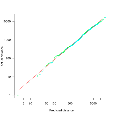
If the data had an exponential distribution the exponent of a fitted power law would be exactly 1. However, the fitted exponent is 1.07, and is statistically significant (for the sample size and standard error of the fit).
The above analysis assumes that the probability of incorrect output,  , is constant. In practice varies across different input values, but over very many inputs is assumed to be clustered around an unchanging average value. It is possible that the input values are divided into two clusters whose incorrect output probabilities are
  and
and  , i.e., a mixture of two exponentials. The worst case scenario is a mixture of umpteen exponentials.
Fitting the distance data to a mixture of two exponentials gives: e^{-0.00037}") (code+data). This corresponds to 10% of the input having an average distance between incorrect output of 482, and 90% having a distance of 2,735 (average 2,482), i.e., one cluster of input values is a lot more likely to produce incorrect output than the other cluster. In the published data the average distance is 2,385.
(code+data). This corresponds to 10% of the input having an average distance between incorrect output of 482, and 90% having a distance of 2,735 (average 2,482), i.e., one cluster of input values is a lot more likely to produce incorrect output than the other cluster. In the published data the average distance is 2,385.
The specification used for the N-version studies came from a study by Nagel and Skrivan who tracked down each of the coding mistakes in the programs tested. They found that around 80% of incorrect outputs were caused by the same coding mistake, and 16% by a second coding mistake (see figure 4.3.7.1-1; an analysis of the Knight & Leveson coding mistakes). Once these two coding mistakes were fixed, other coding mistakes caused incorrect output.
For the LLM generated code, 14 out of the 59 programs had 421 incorrect outputs. Did the LLMs all generate code containing the same coding mistake? I have yet to track down any of the coding mistakes, or get an LLM to do it for me. Once a few coding mistakes have been fixed, ‘allowing’ other coding mistakes to produce incorrect output, will partially correct LLM generated programs stop having correlated failures?
How much does the number of incorrect output change when a different set of random inputs are used?
The random seed used in the published results is: 42. I replicated this output for all 56 programs (it takes around 8.5 hours on my system), and then ran the 1-million inputs on just four programs using the seeds: 101, 20101, 321, 789, and 6000 (which each took around 1-hour). The table below shows the number of incorrect outputs for the various seeds (each numeric column corresponds to a different seed):
Generation information Number of incorrect outputs claude_code__m_claude-haiku-4.5__l_rust 421 432 374 404 424 452 codex__m_gpt-5.1-codex__l_pascal 421 431 372 402 424 451 claude_code__m_claude-sonnet-4.6__l_pascal 1222 1224 1214 1237 1207 1282 codex__m_gpt-5.4-mini__l_python 10052 10063 10181 9944 9963 10122 |
Two (claude_code__m_claude-haiku-4.5__l_rust and codex__m_gpt-5.1-codex__l_pascal) of the 14 programs that had the same number of incorrect outputs with seed 42, had slightly different number of incorrect outputs with other seeds. This suggests that their coding mistakes are slightly different.
All the generated programs had some deviation from the pure single exponential model discussed above.
This simple model for ‘distance’ between incorrect outputs is a good fit to reality because the program performs one basic function and is relatively short (around 500 lines). Larger programs supporting a selection of functionality are going to require much more complicated models.
Sequence generation with no duplicate pairs
Given a fixed set of items (say, 6 A, 12 B and 12 C) what algorithm will generate a randomised sequence containing all of these items with any adjacent pairs being different, e.g., no AA, BB or CC in the sequence? The answer would seem to be provided in my last post. However, turning this bit of theory into practice uncovered a few problems.
Before analyzing the transition matrix approach let’s look at some of the simpler methods that people might use. The most obvious method that springs to mind is to calculate the expected percentage of each item and randomly draw unused items based on these individual item percentages, if the drawn item matches the current end of sequence it is returned to the pool and another random draw is made. The following is an implementation in R:
seq_gen_rand_total=function(item_count) { last_item=0 rand_seq=NULL # Calculate each item's probability item_total=sum(item_count) item_prob=cumsum(item_count)/item_total while (sum(item_count) > 0) { # To recalculate on each iteration move the above two lines here. r_n=runif(1, 0, 1) new_item=which(r_n < item_prob)[1] # select an item if (new_item != last_item) # different from last item? { if (item_count[new_item] > 0) # are there any of these items left? { rand_seq=c(rand_seq, new_item) last_item=new_item item_count[new_item]=item_count[new_item]-1 } } else # Have we reached a state where a duplicate will always be generated? if ((length(which(item_count != 0)) == 1) & (which(item_count != 0)[1] == last_item)) return(0) } return(rand_seq) } |
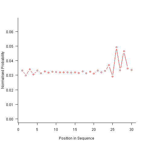
For instance, with 6 A, 12 B and 12 C, the expected probability is 0.2 for A, 0.4 for B and 0.4 for C. In practice if the last item drawn was a C then only an A or B can be selected and the effective probability of A is effectively increased to 0.3333. The red circles in the figure below show the normalised probability of an A appearing at different positions in the sequence of 30 items (averaged over 200,000 random sequences); ideally the normalised probability is 0.0333 for all positions in the sequence In practice the first position has the expected probability (there is no prior item to disturb the probability), the probability then jumps to a higher value and stays sort-of the same until the above-average usage cannot be sustained any more and there is a rapid decline (the sudden peak at position 29 is an end-of-sequence effect I talk about below).
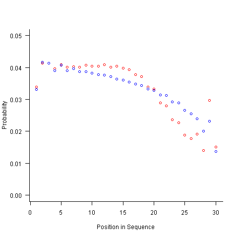
What might be done to get closer to the ideal behavior? A moments thought leads to the understanding that item probabilities change as the sequence is generated; perhaps recalculating item probabilities after each item is generated will improve things. In practice (see blue dots above) the first few items in the sequence have the same probabilities (the slight differences are due to the standard error in the samples) and then there is a sort-of consistent gradual decline driven by the initial above average usage (and some end-of-sequence effects again).
Any sequential generation approach based on random selection runs the risk of reaching a state where a duplicate has to be generated because only one kind of item remains unused (around 80% and 40% respectively for the above algorithms). If the transition matrix is calculated on every iteration it is possible to detect the case when a given item must be generated to prevent being left with unusable items later on. The case that needs to be checked for is when the percentage of one item is greater than 50% of the total available items, when this occurs that item must be generated next, e.g., given (1 A, 1 B, 3 C) a C must be generated if the final list is to have the no-pair property.
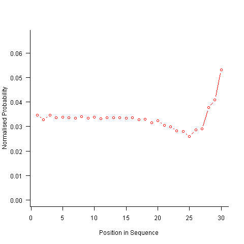
Now the transition matrix approach. Here the last item generated selects the matrix row and a randomly generated value selects the item within the row. Let’s start by generating the matrix once and always using it to select the next item; the resulting normalised probability stays constant for much longer because the probabilities in the transition matrix are not so high that items get used up early in the sequence. There is a small decline near the end and the end-of-sequence effects kick in sooner. Around 55% of generated sequences failed because two of the items were used up early leaving a sequence of duplicates of the remaining item at the end.
Finally, or so I thought, the sought after algorithm using a transition matrix that is recalculated after every item is generated. Where did that oscillation towards the end of the sequence come from?
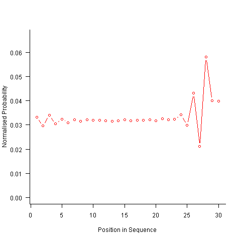
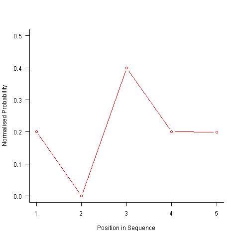
After a some head scratching I realised that the French & Perruchet algorithm is based on redistribution of the expected number of items pairs. Towards the end of the sequence there is a growing probability that the number of remaining As will have dropped to one; it is not possible to create an AA pair from only one A and the assumptions behind the transition matrix calculation break down. A good example of the consequences of this breakdown is the probability distribution for the five item sequences that the algorithm might generate from (1 A, 2 B, 2 C); an A will never appear in position 2 of the sequence:
After various false starts I decided to update the French & Perruchet algorithm to include and end-of-sequence state. This enabled me to adjust the average normalised probability of the main sequence (it has be just right to avoid excess/missing probability inflections at the end), but it did not help much with the oscillations in the last five items (it has to be said that my updated calculations involve a few hand-waving approximations of their own).
I found that a simple, ad hoc solution to damp down the oscillations is to increase any single item counts to somewhere around 1.3 to 1.4. More thought is needed here.
Are there other ways of generating sequences with the desired properties? French & Perruchet give one in their paper; this generates a random sequence, removes one item from any repeating pairs and then uses a random insert and shuffle algorithm to add back the removed items. Robert French responded very promptly to my queries about end-of-sequence effects, sending me a Matlab program implementing an updated version of the algorithm described in the original paper that he tells does not have this problem.
The advantage of the transition matrix approach is that the next item in the sequence can be generated on an as needed basis (provided the matrix is calculated on every iteration it is guaranteed to return a valid sequence if one exists; of course this recalculation removes some randomness for the sequence because what has gone before has some influence of the item distribution that follows). R code used for the above analysis.
I have not been able to locate any articles describing algorithms for generating sequences that are duplicate pair free and would be very interested to hear of any reader experiences.
Transition probabilities when adjacent sequence items must be different
Generating a random sequence from a fixed set of items is a common requirement, e.g., given the items A, B and C we might generate the sequence BACABCCBABC. Often the randomness is tempered by requirements such as each item having each item appear a given number of times in a sequence of a given length, e.g., in a random sequence of 100 items A appears 20 times, B 40 times and C 40 times. If there are rules about what pairs of items may appear in the sequence (e.g., no identical items adjacent to each other), then sequence generation starts to get a bit complicated.
Let’s say we want our sequence to contain: A 6 times, B 12 times and C 12 times, and no same item pairs to appear (i.e., no AA, BB or CC). The obvious solution is to use a transition matrix containing the probability of generating the next item to be added to the end of the sequence based on knowing the item currently at the end of the sequence.
My thinking goes as follows:
- given A was last generated there is an equal probability of it being followed by B or C,
- given B was last generated there is a 6/(6+12) probability of it being followed by A and a 12/(6+12) probability of it being followed by C,
- given C was last generated there is a 6/(6+12) probability of it being followed by A and a 12/(6+12) probability of it being followed by B.
giving the following transition matrix (this row by row approach having the obvious generalization to more items):
                 Second item
               A      B       C
          A    0     .5      .5
First
item      B   .33     0      .67

C .33 .67 0 |
Having read Generating constrained randomized sequences: Item frequency matters by Robert M. French and Pierre Perruchet (from whom I take these examples and algorithm on which the R code is based), I now know this algorithm for generating transition matrices is wrong. Before reading any further you might like to try and figure out why.
The key insight is that the number of XY pairs (reading the sequence left to right) must equal the number of YX pairs (reading right to left) where X and Y are different items from the fixed set (and sequence edge effects are ignored).
If we take the above matrix and multiply it by the number of each item we get the following (if A occurs 6 times it will be followed by B 3 times and C 3 times, if B occurs 12 times it will be followed by A 4 times and C 8 times, etc):
                 Second item
               A      B       C
          A    0      3       3
First
item      B    4      0       8

C 4 8 0 |
which implies the sequence will contain AB 3 times when counted forward and BA 4 times when counted backwards (and similarly for AC/CA). This cannot happen, the matrix is not internally consistent.
The correct numbers are:
                 Second item
               A      B       C
          A    0      3       3
First
item      B    3      0       9

C 3 9 0 |
giving the probability transition matrix:
                 Second item
               A      B       C
          A    0     .5      .5
First
item      B   .25     0      .75

C .25 .75 0 |
This kind of sequence generation occurs in testing and I wonder how many people have made the same mistake as me and scratched their heads over small deviations from the expected results.
The R code to calculate the transition matrix is straight forward but obscure unless you have the article to hand:
# Calculate expression (3) from: # Generating constrained randomized sequences: Item frequency matters # Robert M. French and Pierre Perruchet transition_count=function(item_count) { N_total=sum(item_count) # expected number of transitions ni_nj=(item_count %*% t(item_count))/(N_total-1) diag(ni_nj) = 0 # expected number of repeats d_k=item_count*(item_count-1)/(N_total-1) # Now juggle stuff around to put the repeats someplace else n=sum(ni_nj) n_k=rowSums(ni_nj) s_k=n - 2*n_k R_i=d_k / s_k R=sum(R_i) new_ij=ni_nj*(1-R) + (n_k %*% t(R_i)) + (R_i %*% t(n_k)) diag(new_ij)=0 return(new_ij) } transition_prob=function(item_count) { tc=transition_count(item_count) tp=tc / rowSums(tc) # relies on recycling return(tp) } |
the following calls:
transition_count(c(6, 12, 12)) transition_prob(c(6, 12, 12)) |
return the expected results.
French and Perruchet provide an Excel spreadsheet (note this contains a bug, the formula in cell F20 should start with F5 rather than F6).
Code generation via machine learning
Commercial compiler implementors have to produce compilers that are capable of being used on a typical developer computer. A whole bunch of optimization techniques were known for years but could not be used because few computers had the available memory capacity (in the days when 2M was a lot of memory your author once attended a talk that presented some impressive results and was frustrated to learn that the typical memory footprint was 160M, who would ever imagine developers having so much memory to work within?) These days the available of gigabytes of storage has means that likely computer storage capacity is rarely a reason not to use some optimization technique, although the whole program optimization people are still out in the cold.
What is new these days is the general availability of multiple processors. The obvious use of multiple processors is to have make distribute the compilation load. The more interesting use is having the compiler apply different sets of optimizations techniques on different processors, picking the one that produces the highest quality code.
Optimizing code generation algorithms don’t appear to leave anything to chance and individually they generally don’t. However, selecting an order in which to apply individual optimization algorithms is something of a black art. In some cases code transformations made by one algorithm can interfere with the performance of another algorithm. In some cases the possibility of the interference is known and applies in one direction, choosing the appropriate relative ordering of the two algorithms solves the problem. In other cases the way in which two algorithms interfere with each other depends on the code being translated, now the ordering of the two algorithms becomes problematic. The obvious solution is to try both orderings and pick the one that produces the best result.
Several research groups have investigated the use of machine learning in compiler optimization. cTuning.org is a new project that aims to bring together groups interested in self-tuning adaptive computing systems based on statistical and machine learning techniques.
Commercial pressure is always forcing compiler implementors to produce faster code and use of machine learning techniques can produce some impressive results. Now that multi-processor systems are common it will not be long before compilers writers start to make use of the extra resources now available to them.
The safety critical people have problems trying to show the correctness of compiler output that has been generated by ‘fixed’ algorithms. It is not hard to envisage that in 10 years time all large production quality compilers will be using machine learning.
Readability, an experimental view
Readability is an attribute that source code is often claimed to have, but what is it? While people are happy to use the term they have great difficulty in defining exactly what it is (I will eventually get around discussing my own own views in post). Ray Buse took a very simply approach to answering this question, he asked lots of people (to be exact 120 students) to rate short snippets of code and analysed the results. Like all good researchers he made his data available to others. This posting discusses my thoughts on the expected results and some analysis of the results.
The subjects were first, second, third year undergraduates and postgraduates. I would not expect first year students to know anything and for their results to be essentially random. Over the years, as they gain more experience, I would expect individual views on what constitutes readability to stabilize. The input from friends, teachers, books and web pages might be expected to create some degree of agreement between different students’ view of what constitutes readability. I’m not saying that this common view is correct or bears any relationship to views held by other groups of people, only that there might be some degree of convergence within a group of people studying together.
Readability is not something that students can be expected to have explicitly studied (I’m assuming that it plays an insignificant part in any course marks), so their knowledge of it is implicit. Some students will enjoy writing code and spends lots of time doing it while (many) others will not.
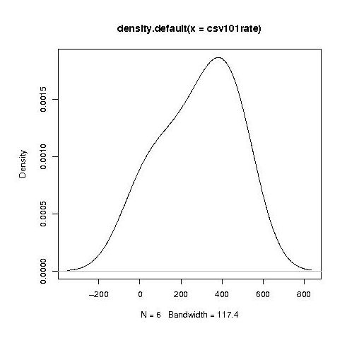
Separating out the data by year the results for first year students look like a normal distribution with a slight bulge on one side (created using plot(density(1_to_5_rating_data)) in R).
year by year this bulge turns (second year):
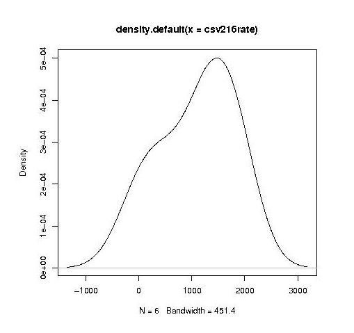
into a hillock (final year):
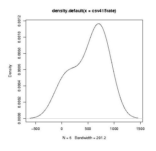
It is tempting to interpret these results as the majority of students assigning an essentially random rating, with a slight positive bias, for the readability of each snippet, with a growing number of more experienced students assigning less than average rating to some snippets.
Do the student’s view converge to a common opinion on readability? The answers appears to be No. An analysis of the final year data using Fleiss’s Kappa shows that there is virtually no agreement between students ratings. In fact every Interrater Reliability and Agreement function I tried said the same thing. Some cluster analysis might enable me to locate students holding similar views.
In an email exchange with Ray Buse I learned that the postgraduate students had a relatively wide range of computing expertise, so I did not analyse their results.
I wish I had thought of this approach to measuring readability. Its simplicity makes it amenable for use in a wide range of experimental situations. The one change I would make is that I would explicitly create the snippets to have certain properties, rather than randomly extracting them from existing source.
Monte Carlo arithmetic operations
Working out whether software based calculations involving floating-point values delivers a sensible answer requires lots of mathematical sophistication and in practice is often impractical or intractable. The vast majority of developers make no effort, indeed most don’t even know why the effort is needed. Various ‘end-user’ solutions have been proposed, e.g., interval arithmetic.
One interesting solution is to perturb the result of floating-point operations and measure the effect on the final answer. Any calculation that is sensitive to small random changes in the result of an operation (there is randomness present in any operation that operates on values that can only be represented to a finite precision) will produce answers that depend on the direction and magnitude of the perturbation. Comparing the answers from several program executions provides a measure of one kind of error present in the calculation.
Monte Carlo arithmetic is a proposed extension of floating-point arithmetic that operates by randomly selecting how round-off errors occur (the proposer provides sample code).
With computing power continuing to increase, running a program several times is often a viable option (we don’t all number crunch for cpu days). Most of the transistors on a modern CPU chip are devoted to memory cache, using a few of these to support Monte Carlo arithmetic instructions is entirely practical. Perhaps when vendors get over supporting the base-10 radix required by the latest IEEE 754R standard and are looking for something new to attract customers they will provide a mechanism that makes it practical to obtain estimates of some of the error in floating-point calculations.
Recent Comments