Archive
Estimating Open source project lifecycle using the Bass model
Is it possible to reliably estimate the elapsed time that a multi-person Open source project spends under major active development, once it has been running for a year or so, and attracted some developers?
The paper Project Life Cycles in Open-Source Software by Das, Ieroshenko, Jain, Qiu, Chin, and Granger fits a Bass diffusion model to the number of monthly developers contributing to a project, and then extrapolates the fitted equation into the future. Is the Bass model a good fit to this kind of data, and how reliable might its prediction be?
What first caught my attention in this paper was the appearance of the sech function (i.e., the hyperbolic secant:  ) in the derived formula. The only other place I have encountered this function in software engineering is the Parr model of project staffing distribution, e.g., effort in hours per week. What’s more, both instances involve
 sech squared, i.e.,  .
.
Is this use of a coincidence, or is there an interesting connection? Let’s look at the paper.
The Bass diffusion model, or just Bass model, assumes that the number of people buying a new product is controlled by two factors: 1) independents who have a constant probability,  , of buying it, and 2) imitators whose probability of purchase depends on
  times the number of existing users of the product (see section 3.6.3 of my book). The Bass model has been extended to handle successive, overlapping generations of a product, e.g., IBM mainframes.
I have not seen the Bass model applied to software lifecycles before (a quick search found a 2014 paper using it to model the time-evolution of package dependencies).
The authors of the new paper introduced sech by normalising two variables in the Bass equation: ^2e^{(p+q)t}}/{(pe^{(p+q)t}+q)^2}")
Time,  is normalised by dividing by time of peak development,
  , and number of developers,
  , is normalised by dividing by peak number of developers,
  , giving:
)") , where
, where ") , and
, and  . It’s not possible to fit this equation to project data because the peak development values are not known (or might not yet have been reached).
The equation in the Parr model is: ") , where the values of
, where the values of  and
and  are obtained by fitting a regression model to project data. The derivation of the Parr model assumes that as project implementation progresses, new problems that need to be solved are discovered (e.g., features to be implemented), an existing problem can spawn at most two new subproblems, and the number of new problems discovered at any time is proportional to the number of remaining problems (cannot find an online version of “An alternative to the Rayleigh curve model for software development effort”).
A connection can be made between the Bass and Parr models by equating the number of developers contributing with the number of problems to be solved, with contributors treated as independents or imitators. The opportunities for potential contributors are likely to increase as a project starts up and then, for some projects decrease (projects such as the Linux kernel just keep on going). The problem implemented by a developer could spawn more than two subproblems.
In practice most of the implementation work on an Open source project is done by a small percentage of developers, with some projects dieing after loosing a few core developers. There is also the issue of the same person contributing using multiple identities.
One method for checking how well a model predicts future measurements is to compare the equations fitted using all the monthly data and, say, the first 75% months. The extent to which both fitted equations agree provides an indication of the likely accuracy of currently unknown future values. The Das et al paper fits the Bass model to the monthly contributor data from 23 projects. The plot below shows the number of monthly developers for numpy (since the project started), along with two fitted Bass models, one for all the data and the other for the first 75% of the data (code+data):
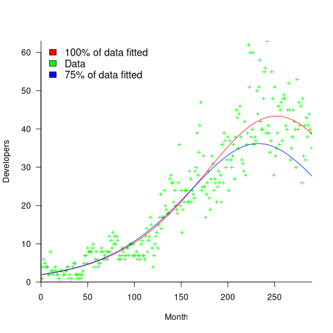
The example project used in the paper has a closer agreement between the two fitted equations, and some of the other projects have much less agreement. The Bass models assumes that monthly contributions are primarily driven by two factors. In practice there could be many other factors driving developer involvement in a project.
Predicting when a project is likely to stop growing is a notoriously difficult problem. Fitting a logistic equation to the growth in lines of code is another example of a model fitting the pattern present in the underlying equation (which flattens off).
It’s possible that weighting developer contribution by the amount of functionality (not lines of code) will produce a closer agreement between theory and practice.
The Putnam project staffing model predates the Parr mode, and later research found that the Putnam model was also a poor predictor of project durations. Both the Parr and Putnam equations can be derived using hazard analysis.
Applying the Bass multi-product generation model to software evolution is now on my to-do list, e.g., use of PHP versions.
Software task estimation using LLMs is fake research
Developers hate having to provide an estimate for the time needed to implement some functionality. Given the extent to which LLMs have become embedded in the software world, offloading the estimation question to an LLM appears to be an obvious solution.
The problem is that LLMs are very unlikely to give a meaningful answer. However, given that 33% of human estimates are accurate (for tasks of a few hours), 66% within a factor of two (over or under), and 95% within a factor of four (over or under), the accuracy bar for LLMs is low.
Given enough training data, LLMs can do amazing things, e.g., help solve difficult maths problems. LLMs often being good-enough at producing source code is dependent on them having been trained on huge amounts of source code.
The miniscule amount of publicly available software task estimation data is orders of magnitude smaller than the quantity needed to effectively fine-tune a software oriented LLM. Estimation training data needs to contain the following information:
- an appropriately detailed description of the problem,
- the source code of the program being updated, as it existed prior to this or any later features being added (similar descriptions may involve different implementation activities on different projects),
- the actual implementation time,
- a summary of the skill set of the developers who did the work (a developer familiar with the source is likely to complete a task faster than a developer new to the project).
There are datasets (here {10K rows} and here {62K rows}) that contain items (1) and (3).
There are datasets (e.g., here {37K rows} and here {23K rows}) that contain (1) for Open source projects, so (2) could be obtained. These datasets contain estimates (usually in Story Points), and a handful of recorded actuals (and often a status change date-time for each issue, which might/perhaps/maybe used as a proxy for actual work time).
Estimation data (in story points, function points, or time) is much more common than Actual (when available, usually time). Needless to say, there are papers (e.g., here and here) that use human estimation data for training, and then measure LLM performance on close it comes to the human estimates, not the actuals.
My 2024 summary of what is known about task estimation did not discuss the impact of LLMs. What was known is 2024 is that several human factors (e.g., use of round numbers and individual risk profile) play a major role in task estimation. LLMs may reduce the time needed for some tasks, but the human factors remain.
The use of round numbers is deeply embedded in the brain. I suspect the impact of LLM usage will not be to reduce implementation time estimates for tasks, but to increase the amount of functionality included in a task to match the established round number times of 1,2,4 and 7 hours.
Users of story points have the option of leaving everything unchanged. However, there are users of story points who equate one story point to one hour. Will the amount of task functionality be increased to maintain this equating?
Users of function points can continue to count them in the same way. What changes, in an LLM world, is the cost of implementing a function point. Given that the method of calculating the number of function points is specified in various national/international standards, it is not possible to simply increase the amount of functionality to maintain the existing price of a function point.
To summarise: LLMs are being trained on small datasets that don’t contain all the required information to give responses that mimic human estimates made in a pre-LLM world.
One of my most popular blog posts is: Software effort estimation is mostly fake research. The adverb “mostly” can be dropped once LLMs are involved.
Remotivating data analysed for another purpose
The motivation for fitting a regression model has a major impact on the model created. Some of the motivations include:
- practicing software developers/managers wanting to use information from previous work to help solve a current problem,
- researchers wanting to get their work published seeks to build a regression model that show they have discovered something worthy of publication,
- recent graduates looking to apply what they have learned to some data they have acquired,
- researchers wanting to understand the processes that produced the data, e.g., the author of this blog.
The analysis in the paper: An Empirical Study on Software Test Effort Estimation for Defense Projects by E. Cibir and T. E. Ayyildiz, provides a good example of how different motivations can produce different regression models. Note: I don’t know and have not been in contact with the authors of this paper.
I often remotivate data from a research paper. Most of the data in my Evidence-based Software Engineering book is remotivated. What a remotivation often lacks is access to the original developers/managers (this is often also true for the authors of the original paper). A complicated looking situation is often simplified by background knowledge that never got written down.
The following table shows the data appearing in the paper, which came from 15 projects implemented by a defense industry company certified at CMMI Level-3.
Proj  Test    Req   Test Meetings Faulty    Actual Scenarios
      Plan    Rev   Env          Scenarios  Effort
      Time          Time
P1    144.5  1.006    85     60     100      2850    270
P2     25.5  1.001    25.5    4       5       250     40
P3     68    1.005    42.5   32      65      1966    185
P4     85    1.002    85    104     150      3750    195
P5    198    1.007   123     87     110      3854    410
P6     57    1.006    35     25      20       903    100
P7    115    1.003    92     55      56      2143    225
P8     81    1.009   156     62      72      1988    287
P9    388    1.004   150    208     553     13246   1153
P10   177    1.008    93     77     157      4012    360
P11    62    1.001   175    186     199      5017    310
P12   111    1.005   116     82     143      3994    423
P13    63    1.009   188    177     151      3914    226
P14    32    1.008    25     28       6       435     63
P15 167 1.001 177 143 510 11555 1133 |
where: TestPlanTime is the test plan creation time in hours, ReqRev is the test/requirements review of period in hours, TestEnvTime is the test environment creation time in hours, Meetings is the number of meetings, FaultyScenarios is the number of faulty test scenarios, Scenarios is the number of Scenarios, and ActualEffort is the actual software test effort.
Industrial data is hard to obtain, so well done to the authors for obtaining this data and making it public. The authors fitted a regression model to estimate software test effort, and the model that almost perfectly fits to actual effort is:
ActualEffort=3190 + 2.65*TestPlanTime
            -3170*ReqRevPeriod - 3.5*TestEnvTime
+10.6*Meetings + 11.6*FaultScrenarios + 3.6*Scenarios |
My reading of this model is that having obtained the data, the authors felt the need to use all of it. I have been there and done that.
Why all those multiplication factors, you ask. Isn’t ActualTime simply the sum of all the work done? Yes it is, but the above table lists the work recorded, not the work done. The good news is that the fitted regression models shows that there is a very high correlation between the work done and the work recorded.
Is there a simpler model that can be used to explain/predict actual time?
Looking at the range of values in each column, ReqRev varies by just under 1%. Fitting a model that does not include this variable, we get (a slightly less perfect fit):
ActualEffort=100  + 2.0*TestPlanTime
                              - 4.3*TestEnvTime
+10.7*Meetings + 12.4*FaultScrenarios + 3.5*Scenarios |
Simple plots can often highlight patterns present in a dataset. The plot below shows every column plotted against every other column (code+data):

Points forming a straight line indicate a strong correlation, and the points in the top-right ActualEffort/FaultScrenarios plot look straight. In fact, this one variable dominates the others, and fits a model that explains over 99% of the deviation in the data:
ActualEffort=550 + 22.5*FaultScrenarios |
Many of the points in the ActualEffort/Screnarios plot are on a line, and adding Meetings data to the model explains just under 99% of the variance in the data:
actualEffort=-529.5
+15.6*Meetings + 8.7*Scenarios |
Given that FaultScrenarios is a subset of Screnarios, this connectedness is not surprising. Does the number of meetings correlate with the number of new FaultScrenarios that are discovered? Questions like this can only be answered by the original developers/managers.
The original data/analysis was interesting enough to get a paper published. Is it of interest to practicing software developers/managers?
In a small company, those involved are likely to already know what these fitted models are telling them. In a large company, the left hand does not always know what the right hand is doing. A CMMI Level-3 certified defense company is unlikely to be small, so this analysis may be of interest to some of its developer/managers.
A usable estimation model is one that only relies on information available when the estimation is needed. The above models all rely on information that only becomes available, with any accuracy, way after the estimate is needed. As such, they are not practical prediction models.
Putnam’s software equation debunked
The implementation of a project has a lifecycle that starts and finishes with zero people working on it. Between starting and finishing, the number of staff quickly grows to a peak before slowly declining. In a series of very hard to obtain papers during the early 1960s (chapter 5), Peter Norden created a large project staffing model described by the Rayleigh equation. This model was evangelized by Lawrence Putnam in the 1970s, who called it the Norden/Rayleigh model, while others sometimes now call it the Norden/Putnam, Putnam/Rayleigh, or some combination of names; Putnam’s papers can be hard to obtain.
The Norden/Rayleigh equation is: 
where:  is work completed,
  is total manpower over the lifespan of the project,
  ,
,  is time of maximum effort per unit time (i.e., the Norden/Rayleigh equation maximum value, which Putnam calls project development time), and is project elapsed time.
Norden’s model is only applicable to large projects (e.g., 2+ man-years), and Putnam points out that the staffing of small projects is usually a square wave, i.e., a number of staff are allocated at the start and this number remains the same until project completion.
As well as evangelizing Norden’s model, Putnam also created his own model; an equation connecting delivered lines of code, total manpower and project duration. The usually cited paper for this work is: “A General Empirical Solution to the Macro Software Sizing and Estimating Problem”, which can sometimes be found as a free download. I had always assumed that people did not take this model seriously, and it was not worth my time debunking it. The paper makes conjures hand-wavy connections between various equations which don’t seem to go anywhere, and eventually connects together a regression equation fitted to nine data points with an observation+assumption about another regression equation to create what Putnam calls the software equation:  , where
  is delivered source code statements, and
  is a constant.
I recently read a 2014 paper by Han Suelmann debunking Putnam’s software equation, which led me to question my assumption about people not using Putnam’s model. Google Scholar shows 1,411 citations, with 133 since 2020. It looks like the software equation is still being taken seriously (or researchers are citing it because everybody else does; a common practice).
Why isn’t Putnam’s software equation worth treating seriously?
First, Putnam’s derivation of the software equation reads like a just-so story based on a tiny amount of data, and second a larger independent dataset does not show the pattern seen in Putnam’s data.
The derivation of the software equation starts by defining productivity as the number of delivered source code statements divided by the total manpower consumed to produce them,  . Ok.
. Ok.
There is more certainty to a line fitted to a set of points that roughly follow a straight line, than to fit a line to points that follow a curve (because there are usually many ‘curve’ equations to choose from). The Norden/Rayleigh equation can be transformed to a form that is amenable to fitting a straight line, i.e., dividing by time and taking logs, as follows (which plugs in the value of  ):
):
=log(K/{t^2_d}) - (1/{2t^2_d})t^2")
Putnam noticed (or perhaps it was the authors of the cited prepublication paper “Software budgeting model” by G. E. P. Box and L. Pallesen, which I cannot locate a copy of) that when plotting ") against
against  : “If the number
  was small, it corresponded with easy systems; if the number was large, it corresponded with hard systems and appeared to fall in a range between these extremes.” Notice that in the screenshot of a figure from Putnam’s paper below, the y-axis is labelled “Difficulty”, not with the quantity actually plotted.
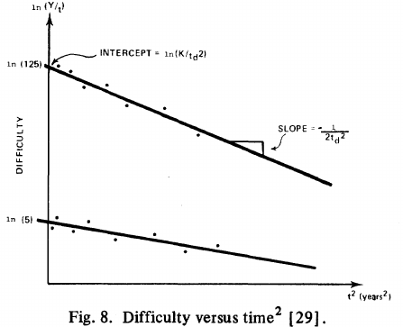
Based on an observation about easy/hard systems (it is never explained how easy/hard is measured) something called difficulty is defined to be:  . No explanation is given for dropping the log scaling, or the possibility that some other relationship might hold.
The screenshot below is of a figure from Putnam’s paper, which plots the values of against for 13 projects. The fitted regression lines (the three lines are fitted using, 9, 2 and 2 points of the 13 projects) have the form  , i.e.,
  (I extracted the points and fitted
  ; code+extracted data):
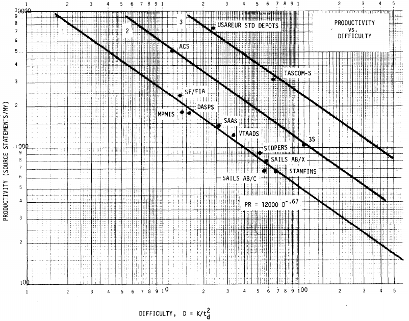
With a bit of algebra, the two equations: and , can be combined to create the software equation.
Yes, Putnam’s software equation was hand-waved into existence by plucking a “difficulty” component from an observation about the behavior of projects in a regression model and equating it to a regression line fitted to nine points.
Are the patterns seen by Putnam found in other projects?
In the 1987 paper “Time-Sensitive Cost Models in the Commercial MIS Environment” D. Ross Jeffery used data from 47 projects to investigate the effort/time relationships used by Putnam to derive his software equation.
The plot below, of log(Difficulty) vs log(Productivity), shows what appears to be a random scattering of points, confirmed by failing to fit a regression model (code+extracted data):

No. The patterns seen by Putnam are not present in these projects. I don’t think that the difference in application domain is relevant (Putnam’s projects were for Military systems and Jeffery’s are for commercial projects). Norden’s model is not specific to software projects.
Jeffery’s uses a regression model to find:  , the corresponding Putnam equation is:
 ^{-2/3}=C_2K^{-0.66}t^1.33_d") (the paper does not include the plot needed to extract the required data). The exponent might be claimed to be close enough, but the exponent is very different.
(the paper does not include the plot needed to extract the required data). The exponent might be claimed to be close enough, but the exponent is very different.
Jeffery’s paper includes a plot of ") against
against ") , and the plot below shows the extracted data (44 points), plus fitted regression line (code+extracted data):
, and the plot below shows the extracted data (44 points), plus fitted regression line (code+extracted data):
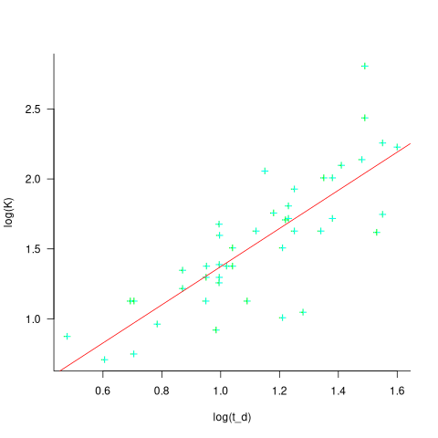
The regression line has the form  . This relationship further undermines assumptions made by Putnam, e.g., smaller systems are easier.
The Han Suelmann paper that triggered this post takes a very different approach to debunking Putnam’s model (he uses simulation to show that random data, drawn from a suitable distribution, can produce the patterns seen by Putnam).
Modelling estimate/actual including uncertainty in the estimate
What is an effective technique for modelling the relationship between the time estimated to implement a task and the actual time taken to implement that task?
A regression model is the obvious approach. However, an important assumption made by the commonly used regression techniques is not met by estimate/actual project data
The commonly used regression techniques involve two kinds of variables: the explanatory variable and the response variable (also known as the independent and dependent variables). For instance, in the equation  ,
,  is the explanatory variable and
  is the response variable.
When fitting a regression model to measurement data, the fitted equation is assumed to have the form such as:  , where
  is uncertainty in the value of , with the valued assumed to have no uncertainty; and
  are constants fitted by the modelling process. The values returned by the model fitting process include an estimate for , as well as estimates for and .
When running an experiment, the values of the explanatory variables(e.g., ) are chosen by the experimenter, with the subject providing the value of the response variable, e.g., .
What does this technical detail have to do with estimation data?
The task estimate/actual values are both provide by the subject (i.e., the developer), there is no experimenter providing one of the values; in fact there is no experiment, these are measurements of things that happened. Both the estimate and actual are response variables, and both contain some amount of uncertainty, and the fitting process needs to take this into account. The appropriate regression technique to use for this case is an errors-in-variables model, which fits the equation +epsilon") , with
, with  being the uncertainty in .
A previous post discussed the surprising behavior that can occur when failing to use errors-in-variables regression for where the data does not contain any explanatory variables, i.e., all the variables contain uncertainty.
The process of fitting an errors-in-variables regression model requires additional input, a value for has to be specified. Taking the example of task estimation, possible uncertainties in the estimate include: misunderstanding of the requirement(s), faded memory of the actual time previously taken by very similar tasks, an inaccurate model of developer skills, and a preference for using round numbers.
What data is available on the uncertainty of individual task estimates? I know of one study where, unknown to them, the individuals estimated the same task twice (in fact, seven people each estimated the same six distinct tasks twice, over a period of three-months). The plot below shows the first/second estimate made by each person for each of the six tasks, with the grey line showing where first==second estimate (code+data):
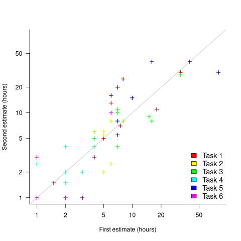
Assuming the estimation uncertainty in this experiment’s data is roughly equal to the estimation uncertainty in other estimation datasets, of tasks taking up to 20 hours, how might it be used to calculate a value for the uncertainty in estimated values?
Two possibilities include:
- Assuming that the uncertainty in both the first and second estimates is equal, a model can be fitted using Deming regression (which treats both variables as having the same uncertainty), and the residual standard error of this model used as the value of . This value for a fitted multiplicative model is 0.6 (code+data),
- using the mean of the relative errors,
}/Est_1") ; its value is 0.55.
; its value is 0.55.
How different are the models built using linear regression and errors-in-variables regression, for small task estimates?
A basic linear regression model fitted to the SiP estimation dataset is:  .
.
Updating this model, using SIMEX, to take into uncertainty in the value of  gives, for an uncertainty error of 0.55:
  , and for an uncertainty error of 0.60:
  . The coefficients for the two models are essentially the same (code+data).
The exponent value is the noticeable difference between the linear regression and errors-in-variables regression models. Adding the assumed amount of uncertainty (based on data from one experiment) to the estimated value leads to a model where estimate/actual are very close to having a linear relationship.
Is this errors-in-variables model any closer to reality than the linear regression model? The model shows that the estimate/actual relationship is closer to linear than was previously thought. Until more data becomes available, we won’t know how close this relationship actually is.
The people who made the estimates in the SiP data also performed the work that took the recorded actual time. Assigning a task to a different person could produce both a different estimate and a different actual, but these possible values are unknown. On a larger scale, different companies bidding on the same contract specify different amounts and have different implementations times; data showing these differences.
A surprising retrospective task estimation dataset
When estimating the time needed to implement a task, the time previously needed to implement similar tasks provides useful guidance. The implementation time for these previous tasks may itself be estimated, because the actual time was not measured or this information is currently unavailable.
How accurate are developer time estimates of previously completed tasks?
I am not aware of any software related dataset of estimates of previously completed tasks (it’s hard enough finding datasets containing information on the actual implementation time). However, I recently found the paper Dynamics of retrospective timing: A big data approach by Balcı, Ünübol, Grondin, Sayar, van Wassenhove, and Wittmann. The data analysed comes from a survey questionnaire, where 24,494 people estimated the how much time they had spent answering the questions, along with recording the current time at the start/end of the questionnaire. The supplementary data is in MATLAB format, and is also available as a csv file in the Blursday database (i.e., RT_Datasets).
Some of the behavior patterns seen in software engineering estimates appear to be general human characteristics, e.g., use of round numbers. An analysis of the estimation performance of a wide sample of the general population could help separate out characteristics that are specific to software engineering and those that apply to the general population.
The following table shows the percentage of answers giving a particular Estimate and Actual time, in minutes. Over 60% of the estimates are round numbers. Actual times are likely to be round numbers because people often give a round number when asked the time (code+data):
   Minutes    Estimate    Actual
     20          18%       8.5%
     15          15%       5.3%
     30          12%       7.6%
     25          10%       6.2%
10 7.7% 2.1% |
I was surprised to see that the authors had fitted a regression model with the Actual time as the explanatory variable and the Estimate as the response variable. The estimation models I have fitted always have the roles of these two variables reversed. More of this role reversal difference below.
The equation fitted to the data by the authors is (they use the term Elapsed, for consistency with other blog articles I continue to use Actual; code+data):

This equation says that, on average, for shorter Actual times the Estimate is higher than the Actual, while for longer Actual times the average Estimate is lower.
Switching the roles of the variables, I expected to see a fitted model whose coefficients are somewhat similar to the algebraically transformed version of this equation, i.e.,  . At the very least, I expected the exponent to be greater than one.
Surprisingly, the equation fitted with the variables roles reversed is very similar, i.e., the equations are the opposite of each other:

This equation says that, on average, for shorter Estimate times the Actual time is higher than the Estimate, while for longer Estimate times the average Actual is lower, i.e., the opposite behavior specifie dby the earlier equation.
I spent some time trying to understand how it was possible for data to be fitted such that (x ~ y) == (y ~ x), even posting a question to Cross Validated. I might, in a future post, discuss the statistical issues behind this behavior.
So why did the authors of this paper treat Actual as an explanatory variable?
After a flurry of emails with the lead author, Fuat Balcı (who was very responsive to my questions), where we both doubled checked the code/data and what we thought was going on, Fuat answered that (quoted with permission):
“The objective duration is the elapsed time (noted by the experimenter based on a clock reading), and the estimate is the participant’s response. According to the psychophysical approach the mapping between objective and subjective time can be defined by regressing the subjective estimates of the participants on the objective duration noted by the experimenter. Thus, if your research question is how human’s retrospective experience of time changes with the duration of events (e.g., biases in time judgments), the y-axis should be the participant’s response and the x-axis should be the actual duration.”
This approach has a logic to it, and is consistent with the regression modelling done by other researchers who study retrospective time estimation.
So which modelling approach is correct, and are people overestimating or underestimating shorter actual time durations?
Going back to basics, the structure of this experiment does not produce data that meets one of the requirements of the statistical technique we are both using (ordinary least squares) to fit a regression model. To understand why ordinary least squares, OLS, is not applicable to this data, it’s necessary to delve into a technical detail about the mathematics of what OLS does.
The equation actually fitted by OLS is:  , where is an error term (i.e., ‘noise’ caused by all the effects other than ). The value of is assumed to be exact, i.e., not contain any ‘noise’.
Usually, in a retrospective time estimation experiment, subjects hear, for instance, a sound whose duration is decided in advance by the experimenter; subjects estimate how long each sound lasted. In this experimental format, it makes sense for the Actual time to appear on the right-hand-side as an explanatory variable and for the Estimate response variable on the left-hand-side.
However, for the questionnaire timing data, both the Estimate and Actual time are decided by the person giving the answers. There is no experimenter controlling one of the values. Both the Estimate and Actual values contain ‘noise’. For instance, on a different day a person may have taken more/less time to actually answer the questionnaire, or provided a different estimate of the time taken.
The correct regression fitting technique to use is errors-in-variables. An errors-in-variables regression fits the equation:  + epsilon") , where:
, where:  is the true value of and is its associated error. A selection of packages are available for fitting a variety of errors-in-variables models.
I regularly see OLS used in software engineering papers (including mine) where errors-in-variables is the technically correct technique to use. Researchers are either unaware of the error issues or assuming that the difference is not important. The few times I have fitted an errors-in-variables model, the fitted coefficients have not been much different from those fitted by an OLS model; for this dataset the coefficient difference is obviously important.
The complication with building an errors-in-variables model is that values need to be specified for the error terms and . With OLS the value of is produced as part of the fitting process.
How might the required error values be calculated?
If some subjects round reported start/stop times, there may not be any variation in reported Actual time, or it may jump around in 5-minute increments depending on the position of the minute hand on the clock.
Learning researchers have run experiments where each subject performs the same task multiple times. Performance improves with practice, which makes it difficult to calculate the likely variability in the first-time performance. If we assume that performance is skill based, the standard deviation of all the subjects completing within a given timeframe could be used to calculate an error term.
With 60% of Estimates being round numbers, there might not be any variation for many people, or perhaps the answer given will change to a different round number. There is Estimate data for different, future tasks, and a small amount of data for the same future tasks. There is data from many retrospective studies using very short time intervals (e.g., tens of seconds), which might be applicable.
We could simply assume that the same amount of error is present in each variable. Deming regression is an errors-in-variables technique that supports this approach, and does not require any error values to be specified. The following equations have been fitted using Deming regression (code+data):

and

While these two equations are consistent with each other, we don’t know if the assumption of equal errors in both variables is realistic.
What next?
Hopefully it will be possible to work out reasonable error values for the Actual/Estimate times. Fitting a model using these values will tell us wether any over/underestimating is occurring, and the associated span of time durations.
I also need to revisit the analysis of software task estimation times.
What is known about software effort estimation in 2024
It’s three years since my 2021 post summarizing what I knew about estimating software tasks. While no major new public datasets have appeared (there have been smaller finds), I have talked to lots of developers/managers about the findings from the 2019/2021 data avalanche, and some data dots have been connected.
A common response from managers, when I outline the patterns found, is some variation of: “That sounds about right.” While it’s great to have this confirmation, it’s disappointing to be telling people what they already know, even if I can put numbers to the patterns.
Some of the developer behavior patterns look, to me, to be actionable, e.g., send developers on a course to unbias their estimates. In practice, managers are worried about upsetting developers or destabilising teams. It’s easy for an unhappy developer to find another job (the speakers at the meetups I attend often end by saying: “and we’re hiring.”)
This post summarizes a talk I gave recently on what is known about software estimating; a video will eventually appear on the British Computer Society‘s Software Practice Advancement group’s YouTube channel, and the slides are on Github.
What I call the historical estimation models contain source code, measured in lines, as a substantial component, e.g., COCOMO which overfits a miniscule dataset. The problem with this approach is that estimates of the LOC needed to implement some functionality LOC are very inaccurate, and different developers use different LOC to implement the same functionality.
Most academic research in software effort estimation continues to be based on miniscule datasets; it’s essentially fake research. Who is doing good research in software estimating? One person: Magne Jørgensen.
Almost all the short internal task estimate/actual datasets contain all the following patterns:
- use of round-numbers (known as heaping in some fields). The ratios of the most frequently used round numbers, when estimating time, are close to the ratios of the Fibonacci sequence,
- short tasks tend to be under-estimated and long tasks over-estimate. Surprisingly, the following equation is a good fit for many time-based datasets:
 ,
, - individuals tend to either consistently over or under estimate (this appears to be connected with the individual’s risk profile),
- around 30% of estimates are accurate, 68% within a factor of two, and 95% within a factor of four; one function point dataset, one story point dataset, many time datasets,
- developer estimation accuracy does not change with practice. Possible reasons for this include: variability in the world prevents more accurate estimates, developers choose to spend their learning resources on other topics (such as learning more about the application domain).
I have a new ChatGPT generated image for my slide covering the #Noestimates movement:

Estimation accuracy in the (building|road) construction industry
Lots of people complain about software development taking longer than estimated. Are estimates in other industries more accurate, and do they contain patterns similar to those seen in software task estimates?
Readers will probably not be surprised to learn that obtaining estimate/actual data is as hard for other industries as it is for software.
Software engineering sometimes gets compared with building construction, in the sense that building construction is perceived as being straightforward and predictable. My tiny experience with building construction is that it is not as straightforward and predictable as outsiders think, a view echoed by the few people in the building industry I have spoken to.
I have found two building datasets, the supplementary material from: Forecasting the Project Duration Average and Standard Deviation from Deterministic Schedule Information (the 101 rows also include some service projects), and Ballesteros-Pérez kindly sent me the data for Duration and Cost Variability of Construction Activities: An Empirical Study which included 746 rows of road construction estimate/actual data from an unknown source. This data is for large projects, where those involved had to bid to get the work.
The following plot reminds us of how effort vs actual often looks like for short software tasks; it includes a fitted regression model and prediction intervals at one standard deviation (68.3%) and two standard deviations (95%); the faint grey line shows Estimate == Actual (post discussing the analysis and linking to code+data):
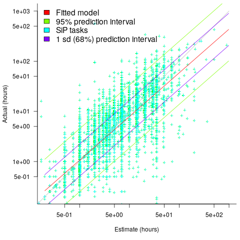
The data in the above plot is for small tasks, which did not involve bidding for the work.
The following plot shows estimated vs actual duration for 101 construction projects. The red line has the form:  , i.e., average estimate is 9% lower than actual duration (blue line shows
  ; code+data).
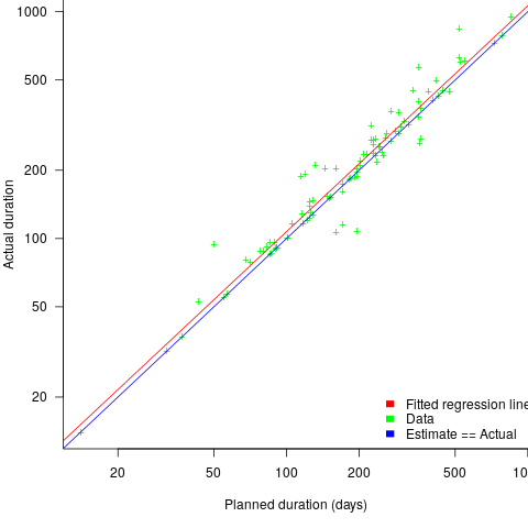
The obvious differences are that the fitted line shows consistent underestimation (hardly surprising when bidding for work; 16% of estimates are greater than the actual), that the variance of project estimate/actual about the line is much smaller for building construction, and that the red/blue lines are essentially parallel (the exponent for software tasks is consistently around 0.85, rather than 1)
The following plot shows estimated vs actual for 746 road construction projects. The red line has the form:  , i.e., average estimate is 24% lower than actual duration (blue line shows ; code+data):
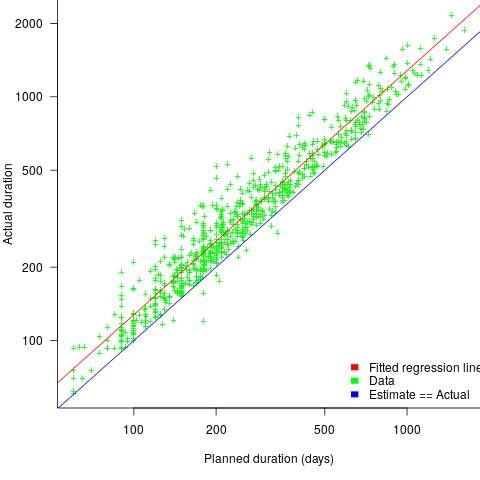
Again there is a consistent average underestimate (project bidding was via an auction process), the red/blue lines are essentially parallel, and while the estimate/actual variance is larger than for building construction only 1.5% estimates are greater than the actual.
Consistent underestimating is not surprising for external projects awarded via a bidding process.
The unpredicted differences are the much smaller estimate/actual variance (compared to software), and the fitted line running parallel to .
Estimating quantities from several hundred to several thousand
How much influence do anchoring and financial incentives have on estimation accuracy?
Anchoring is a cognitive bias which occurs when a decision is influenced by irrelevant information. For instance, a study by John Horton asked 196 subjects to estimate the number of dots in a displayed image, but before providing their estimate subjects had to specify whether they thought the number of dots was higher/lower than a number also displayed on-screen (this was randomly generated for each subject).
How many dots do you estimate appear in the plot below?

Estimates are often round numbers, and 46% of dot estimates had the form of a round number. The plot below shows the anchor value seen by each subject and their corresponding estimate of the number of dots (the image always contained five hundred dots, like the one above), with round number estimates in same color rows (e.g., 250, 300, 500, 600; code+data):
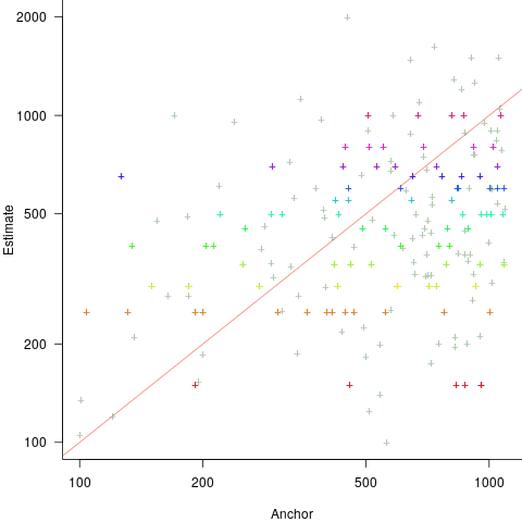
How much influence does the anchor value have on the estimated number of dots?
One way of measuring the anchor’s influence is to model the estimate based on the anchor value. The fitted regression equation  explains 11% of the variance in the data. If the higher/lower choice is included the model, 44% of the variance is explained; higher equation is:
  and lower equation is:
  (a multiplicative model has a similar goodness of fit), i.e., the anchor has three-times the impact when it is thought to be an underestimate.
How much would estimation accuracy improve if subjects’ were given the option of being rewarded for more accurate answers, and no anchor is present?
A second experiment offered subjects the choice of either an unconditional payment of $2.50 or a payment of $5.00 if their answer was in the top 50% of estimates made (labelled as the risk condition).
The 196 subjects saw up to seven images (65 only saw one), with the number of dots varying from 310 to 8,200. The plot below shows actual number of dots against estimated dots, for all subjects; blue/green line shows  , and red line shows the fitted regression model
  (code+data):
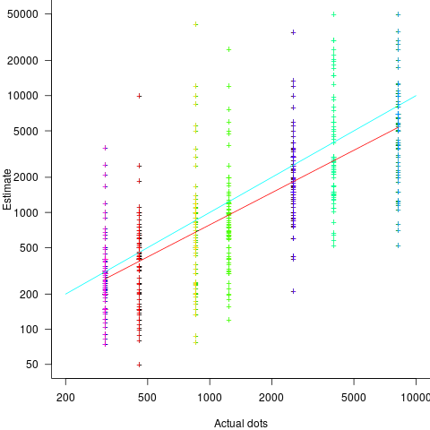
The variance in the estimated number of dots is very high and increases with increasing actual dot count, however, this behavior is consistent with the increasing variance seen for images containing under 100 dots.
Estimates were not more accurate in those cases where subjects chose the risk payment option. This is not surprising, performance improvements require feedback, and subjects were not given any feedback on the accuracy of their estimates.
Of the 86 subjects estimating dots in three or more images, 44% always estimated low and 16% always high. Subjects always estimating low/high also occurs in software task estimates.
Estimation patterns previously discussed on this blog have involved estimated values below 100. This post has investigated patterns in estimates ranging from several hundred to several thousand. Patterns seen include extensive use of round numbers and increasing estimate variance with increasing actual value; all seen in previous posts.
NoEstimates panders to mismanagement and developer insecurity
Why do so few software development teams regularly attempt to estimate the duration of the feature/task/functionality they are going to implement?
Developers hate giving estimates; estimating is very hard and estimates are often inaccurate (at a minimum making the estimator feel uncomfortable and worse when management treats an estimate as a quotation). The future is uncertain and estimating provides guidance.
Managers tell me that the fear of losing good developers dissuades them from requiring teams to make estimates. Developers have told them that they would leave a company that required them to regularly make estimates.
For most of the last 70 years, demand for software developers has outstripped supply. Consequently, management has to pay a lot more attention to the views of software developers than the views of those employed in most other roles (at least if they want to keep the good developers, i.e., those who will have no problem finding another job).
It is not difficult for developers to get a general idea of how their salary, working conditions and practices compares with other developers in their field/geographic region. They know that estimating is not a common practice, and unless the economy is in recession, finding a new job that does not require estimation could be straight forward.
Management’s demands for estimates has led to the creation of various methods for calculating proxy estimate values, none of which using time as the unit of measure, e.g., Function points and Story points. These methods break the requirements down into smaller units, and subcomponents from these units are used to calculate a value, e.g., the Function point calculation includes items such as number of user inputs and outputs, and number of files.
How accurate are these proxy values, compared to time estimates?
As always, software engineering data is sparse. One analysis of 149 projects found that  , with the variance being similar to that found when time was estimated. An analysis of Function point calculation data found a high degree of consistency in the calculations made by different people (various Function point organizations have certification schemes that require some degree of proficiency to pass).
Managers don’t seem to be interested in comparing estimated Story points against estimated time, preferring instead to track the rate at which Story points are implemented, e.g., velocity, or burndown. There are tiny amounts of data comparing Story points with time and Function points.
The available evidence suggests a relationship connecting Function points to actual time, and that Function points have similar error bounds to time estimates; the lack of data means that Story points are currently just a source of technobabble and number porn for management power-points (send me Story point data to help change this situation).
Recent Comments