Archive
Predicting reports of new faults by counting past reports
One of the many difficulties of estimating the probability of a previously unseen fault being reported is lack of information on the amount of time spent using the application; the more time spent, the more likely a previously unseen/seen fault will be experienced. Formal prerelease testing is one of the few situations where running time is likely to be recorded.
Information that is sometimes available is the date/time of fault reports. I say sometimes because a common response to an email asking researchers for their data, is that they did not record information about duplicate faults.
What information might possibly be extracted from a time ordered list of all reported faults, i.e., including reports of previously reported faults?
My starting point for answering this questions is a previous post that analysed time to next previously unreported fault.
The following analysis treats the total number of previously reported faults as a proxy for a unit of time. The LLMs used were Deepseek (which continues to give high quality responses, which are sometimes wrong), Kimi (which is working well again, after 6–9 months of poor performance and low quality chain of thought output), ChatGPT (which now produces good quality chain of thought), Grok (which has become expressive, if not necessarily more accurate), and for the first time GLM 5.1 from the company Z.ai.
After some experimentation, the easiest to interpret formula was obtained by modelling the ‘time’ between occurrences of previously unreported faults. The following is the prompt used (this models each fault as a process that can send a signal, with the Poisson and exponential distribution requirements derived from experimental evidence; here and here):
There are $N$ independent processes. Each process, $P_i$, transmits a signal, and the number of signals transmitted in a fixed time interval, $T$, has a Poisson distribution with mean $L_i$ for $1<= i <= N$. The values $L_i$ are randomly drawn from the same exponential distribution. What is the expected number of signals transmitted by all processes between the $k$ and $k+1$ first signals from the $N$ processes. |
The LLMs responses were either (based on a weekend studying the LLM chain-of-thought response): correct (GLM), very close (ChatGPT made an assumption that was different from the one made by GLM; after some back and forth prompts between the models (via me typing them), ChatGPT agreed that GLM’s assumption was the correct one), wrong but correct when given some hints (Grok without extra help goes down a Polya urn model rabbit hole), and always wrong (Deepseek, and Kimi, which normally do very well).
The expected number of previously reported faults between the  ‘th and
 ") ‘th first occurrence of an unreported fault, is:
‘th first occurrence of an unreported fault, is:
![E[F_{prev}]={k*(2N-k-1)}/{(N-k)(N-k-1)}](https://shape-of-code.com/wp-content/plugins/wpmathpub/phpmathpublisher/img/math_977_e350e5adb969b64ebc06610cb57dd38d.png "E[F_{prev}]={k*(2N-k-1)}/{(N-k)(N-k-1)}") , where
, where  is the total number of possible distinct fault reports.
The variance is: (2(N-k)^2+(k-1)(N-k)+2(k-1))}/{(N-k)^2(N-k-1)^2(N-k-2)}")
While is unknown, but there is a distinctive shape to the plot of the change in the expected number of reports against (expressed as a percentage of ), as the plot below shows (see red line; code+data):
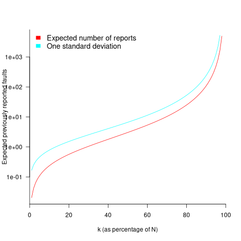
Perhaps, for a particular program, it is possible to estimate as a percentage of by comparing the relative change in the number of previously reported faults that occur between pairs of previously unreported faults.
Unfortunately the variance in the number previously reported faults completely swamps the expected value, ![E[F_{prev}]](https://shape-of-code.com/wp-content/plugins/wpmathpub/phpmathpublisher/img/math_981.5_a5ef61e64e07d16ba49517a817b2a39a.png "E[F_{prev}]") . The blue/green line in the plot above shows the upper bound of one standard deviation, with the lower bound being zero. In other words, any value between zero and the blue/green line is within one standard deviation of the expected value. There is no possibility of reliably narrowing down the bounds for , based on an estimated position of on the red curve above 🙁
. The blue/green line in the plot above shows the upper bound of one standard deviation, with the lower bound being zero. In other words, any value between zero and the blue/green line is within one standard deviation of the expected value. There is no possibility of reliably narrowing down the bounds for , based on an estimated position of on the red curve above 🙁
To quote GLM: “The variance always exceeds the mean because of two layers of randomness: the Poisson shot noise and the uncertainty in the rates themselves.”
That is the theory. Since data is available (i.e., duplicate fault reports in Apache, Eclipse and KDE), allowing the practice to be analysed (code+data).
The above analysis assumes that the software is a closed system (i.e., no code is added/modified/deleted), and that the fault report system does not attempt to reduce duplicate reports (e.g., by showing previously reported problems that appear to be similar, so the person reporting the problem may decide not to report it).
The closed system issue can be handled by analysing individual versions, but there is no solution to duplicate report reduction systems.
Across all KDE projects around 7% of reported problems were duplicates (code+data). For specific fault classes the percentage is often lower, e.g., for the konqueror project 2% of reports deal with program crashing.
Fuzzing is another source of duplicate reports. However, fuzzers are explicitly trying to exercise all parts of the code, i.e., the input is consistently different (or is intended to be).
Summary. This analysis provides another nail in the coffin of estimating the probability of encountering a previously unseen fault and of estimating the number of fault report experiences contained in a program.
Extracting information from duplicate fault reports
Duplicate fault reports (that is, reports whose cause is the same underlying coding mistake) are an underused source of information. I sometimes email the authors of a paper analysing fault data asking for information about duplicates. Duplicate information is rarely available, because the authors don’t bother to record it.
If a program’s coding mistakes are a closed population, i.e., no new ones are added or existing ones fixed, duplicate counts might be used to estimate the number of remaining mistakes.
However, coding mistakes in production software systems are invariably open populations, i.e., reported faults are fixed, and new functionality (containing new coding mistakes) is added.
A dataset made available by Sadat, Bener, and Miranskyy contains 18 years worth of information on duplicate fault reports in Apache, Eclipse and KDE. The following analysis uses the KDE data.
Fault reports are created by users, and changes in the rate of reports whose root cause is the same coding mistake provides information on changes in the number of active users, or changes in the functionality executed by the active users. The plot below shows, for 10 unique faults (different colors), the number of days between the first report and all subsequent reports of the same fault (plus character); note the log scale y-axis (code+data):

Changes in the rate at which duplicates are reported are visible as changes in the slope of each line formed by plus signs of the respective color. Possible reasons for the change include: the coding mistake appears in a new release which users do not widely install for some time, 2) a fault become sufficiently well known, or workaround provided, that the rate of reporting for that fault declines. Of course, only some fault experiences are ever reported.
Almost all books/papers on software reliability that model the occurrence of fault experiences treat them as-if they were a Non-Homogeneous Poisson Process (NHPP); in most cases, authors are simply repeating what they have read elsewhere.
Some important assumptions made by NHPP models do not apply to software faults. For instance, NHPP models assume that the probability of encountering a fault experience is the same for different coding mistakes, i.e., they are all equally likely. What does the evidence show about this assumption? If all coding mistakes had the same probability of producing a fault experience, the mean time between duplicate fault reports would be the same for all fault reports. The plot below shows the interval, in days, between consecutive duplicate fault reports, for the 392 faults whose number of duplicates was between 20 and 100, sorted by interval (out of a total of 30,377; code+data):
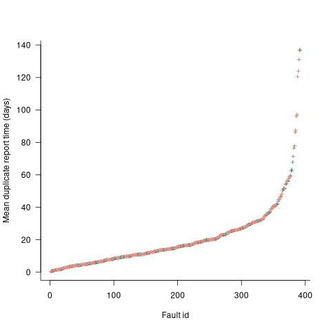
The variation in mean time between duplicate fault reports, for different faults, is evidence that different coding mistakes have different probabilities of producing a fault experience. This behavior is consistent with the observation that mistakes in deeply nested if-statements are less likely to be executed than mistakes contained in less-deeply nested code. However, this observation invalidating assumptions made by NHPP models has not prevented them dominating the research literature.
Analysis of when refactoring becomes cost-effective
In a cost/benefit analysis of deciding when to refactor code, which variables are needed to calculate a good enough result?
This analysis compares the excess time-code of future work against the time-cost of refactoring the code. Refactoring is cost-effective when the reduction in future work time is less than the time spent refactoring. The analysis finds a relationship between work/refactoring time-costs and number of future coding sessions.
Linear, or supra-linear case
Let’s assume that the time needed to write new code grows at a linear, or supra-linear rate, as the amount of code increases ( ):
):

where:  is the base time for writing new code on a freshly refactored code base,
  is the number of lines of code that have been written since the last refactoring, and
  and
and  are constants to be decided.
The total time spent writing code over  sessions is:
^x}")
If the same number of new lines is added in every coding session,  , and is an integer constant, then the sum has a known closed form, e.g.:
x=1, ^1}={n(n+1)}/2L_s") ; x=2,
; x=2, ^2}={n(n+1)(2n+1)}/6{L_s}^2")
Let’s assume that the time taken to refactor the code written after sessions is:
^y")
where:  and
and  are constants to be decided.
The reason for refactoring is to reduce the time-cost of subsequent work; if there are no subsequent coding sessions, there is no economic reason to refactor the code. If we assume that after refactoring, the time taken to write new code is reduced to the base cost, , and that we believe that coding will continue at the same rate for at least another  sessions, then refactoring existing code after sessions is cost-effective when:
^y < k_1sum{i=n+1}{n+f}{(iL_s)^x}")
assuming that is much smaller than , setting  , and rearranging we get:

after rearranging we obtain a lower limit on the number of future coding sessions, , that must be completed for refactoring to be cost-effective after session ::

It is expected that  ; the contribution of code size, at the end of every session, in the calculation of
  and
and  is equal (i.e.,
 ^y") ), and the overhead of adding new code is very unlikely to be less than refactoring all the newly written code.
), and the overhead of adding new code is very unlikely to be less than refactoring all the newly written code.
With  ,
,  must be close to zero; otherwise, the likely relatively large value of (e.g., 100+) would produce surprisingly high values of .
Sublinear case
What if the time overhead of writing new code grows at a sublinear rate, as the amount of code increases?
Various attributes have been found to strongly correlate with the  of lines of code. In this case, the expressions for and become:

")
and the cost/benefit relationship becomes:
 < k_1sum{i=n+1}{n+f}{log(iL_s)}")
applying Stirling’s approximation and simplifying (see Exact equations for sums at end of post for details) we get:
 < k_1(f(log(n+f)-1)+f log{L_s})")
+log{L_s}-1} < f")
applying the series expansion (for  ):
):  , we get
 < f")
Discussion
What does this analysis of the cost/benefit relationship show that was not obvious (i.e., the relationship  is obviously true)?
What the analysis shows is that when real-world values are plugged into the full equations, all but two factors have a relatively small impact on the result.
A factor not included in the analysis is that source code has a half-life (i.e., code is deleted during development), and the amount of code existing after sessions is likely to be less than the  used in the analysis (see Agile analysis).
As a project nears completion, the likelihood of there being more coding sessions decreases; there is also the every present possibility that the project is shutdown.
The values of and encode information on the skill of the developer, the difficulty of writing code in the application domain, and other factors.
Exact equations for sums
The equations for the exact sums, for  , are:
")
+1)")
(2n(n+1)+2fn+f+f^2)")
-zeta(-0.5, f+n+1)") , where
, where  is the Hurwitz zeta function.
Sum of a log series: !}/{n!}}+f log{L_s}")
using Stirling’s approximation we get
!)}-log(n!) approx (n+f-0.5)log(n+f)-(n+f)-((n-0.5)log n-n)")
simplifying
!)}-log(n!) approx (n-0.5)log(1+f/n)+f log(n+f)-f")
and assuming that is much smaller than gives
!)}-log(n!) approx f(log(n+f)-1)")
Update
The analysis above assumes that the time contribution of the base rate, , is independent of the changes,  . The following analysis combines these two contributions into a single rate:
L)^b}")
where:  ,
,  , , and are positive constants, with
  , and
, and  .
.
The following is a very good approximation to this sum (thanks to Grok 4.1 beta; chat script):
L})")
where: L")
Complex software makes economic sense
Economic incentives motivate complexity as the common case for software systems.
When building or maintaining existing software, often the quickest/cheapest approach is to focus on the features/functionality being added, ignoring the existing code as much as possible. Yes, the new code may have some impact on the behavior of the existing code, and as new features/functionality are added it becomes harder and harder to predict the impact of the new code on the behavior of the existing code; in particular, is the existing behavior unchanged.
Software is said to have an attribute known as complexity; what is complexity? Many definitions have been proposed, and it’s not unusual for people to use multiple definitions in a discussion. The widely used measures of software complexity all involve counting various attributes of the source code contained within individual functions/methods (e.g., McCabe cyclomatic complexity, and Halstead); they are all highly correlated with lines of code. For the purpose of this post, the technical details of a definition are glossed over.
Complexity is often given as the reason that software is difficult to understand; difficult in the sense that lots of effort is required to figure out what is going on. Other causes of complexity, such as the domain problem being solved, or the design of the system, usually go unmentioned.
The fact that complexity, as a cause of requiring more effort to understand, has economic benefits is rarely mentioned, e.g., the effort needed to actively use a codebase is a barrier to entry which allows those already familiar with the code to charge higher prices or increases the demand for training courses.
One technique for reducing the complexity of a system is to redesign/rework its implementation, from a system/major component perspective; known as refactoring in the software world.
What benefit is expected to be obtained by investing in refactoring? The expected benefit of investing in redesign/rework is that a reduction in the complexity of a system will reduce the subsequent costs incurred, when adding new features/functionality.
What conditions need to be met to make it worthwhile making an investment,  , to reduce the complexity, , of a software system?
Let’s assume that complexity increases the cost of adding a feature by some multiple (greater than one). The total cost of adding features is:

where:  is the system complexity when feature
  is added, and
  is the cost of adding this feature if no complexity is present.
 ,
,  , …
, … 
where:  is the base complexity before adding any new features.
Let’s assume that an investment, , is made to reduce the complexity from  (with
(with  ) to
) to  , where
  is the reduction in the complexity achieved. The minimum condition for this investment to be worthwhile is that:
 or
or 
where:  is the total cost of adding new features to the source code after the investment, and
  is the total cost of adding the same new features to the source code as it existed immediately prior to the investment.
Resetting the feature count back to  , we have:
*F_1+(C_B+C_N+C_2)*F_2+...+(C_B+C_N+C_m)*F_m")
and
*F_1+(C_B+C_N-C_R+C_2)*F_2+...+(C_B+C_N-C_R+C_m)*F_m")
and the above condition becomes:
-(C_B+C_N-C_R+C_1))*F_1+...+((C_B+C_N+C_m)-(C_B+C_N-C_R+C_m))*F_m")


The decision on whether to invest in refactoring boils down to estimating the reduction in complexity likely to be achieved (as measured by effort), and the expected cost of future additions to the system.
Software systems eventually stop being used. If it looks like the software will continue to be used for years to come (software that is actively used will have users who want new features), it may be cost-effective to refactor the code to returning it to a less complex state; rinse and repeat for as long as it appears cost-effective.
Investing in software that is unlikely to be modified again is a waste of money (unless the code is intended to be admired in a book or course notes).
Maths GCE from 1972 (paper 2)
While sorting through some old papers I came across my GCE maths O level exam papers from the summer of 1972. They are known as GCSE exams these days and are taken by 16 year olds at the end of their final year of compulsory education in the UK. I was lucky enough to have a maths teacher who believed in encouraging students to excel and I (plus five others) took this exam when we were 15. I never got the chance to thank Mr Merritt for the profound effect he had on my life.
For many years the average grades achieved by students in the UK has had a steady upward trend and some people claim the exams are getting easier (others that students are better taught, or at least better taught to pass exams). These days students have calculators and don’t use log tables, so question 3 of Section A is not applicable.
Exam papers in the UK are written by various examining boards. Mine were from the University of London, Syllabus D. I have two papers labeled “Mathematics 2” and “Mathematics 3” and don’t recall if there was ever a “Mathematics 1”. The following are the questions from “Mathematics 2”.
All necessary working must be shown.
- Factorise

Hence, or otherwise, find the exact value of
")
4 marks
- Given that
}") , express in terms of
, express in terms of  and
and  .
.
3 marks
- Use four digit tables to evaluate
}") .
.
4 marks
- Given that
 is a factor of
  , calculate the value of .
3 marks
-
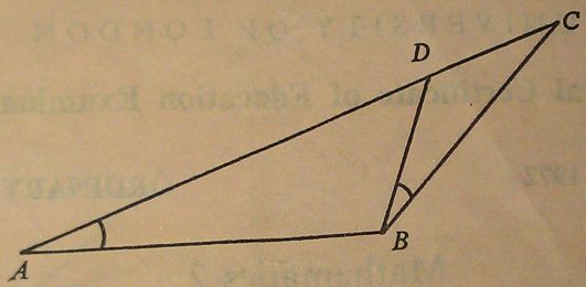
In the diagram ∠DBC = ∠BAD and ADC is a straight line. State which of the two triangles are similar.
If AB = 7 cm, BC = 6 cm and DC = 4 cm, calculate the lengths of AC and BD.
5 marks
- A bicycle wheel has diameter 35 cm. Calculate how many revolutions it makes every minute when the bicycle is travelling at 33 km/h. [ Take
 as 22/7 ]
4 marks
- Calculate the gradient of the curve
 at the point (1, -5). Calculate also the coordinates of the point on the curve where the gradient is 1.
4 marks
-
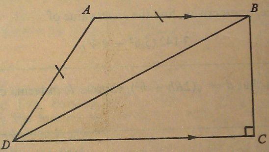
In the diagram, AB is parallel to DC, AB = AD and ∠C = 90°. Prove that ∠DAB = 2∠DBC.
5 marks
as 3.142 when required- A ship is at the point P (54°N, 55°W). Calculate the distance, in nautical miles, of P from the equator.
The ship then sails 500 nautical miles due East to a point Q. Calculate the latitude and longitude of Q.
An aircraft flies due South at a constant height of 10 000 m from the point vertically above P to a point vertically above the equator. Taking the earth to be a sphere of radius 6 370 km, calculate the length of the arc along which the aircraft flies.
17 marks
- Draw a circle of radius 5.5 cm. Using ruler and compasses only, construct a tangent to the circle at any point A on its circumference.
Using a protractor, construct the points A, B and C on this circle so that the angles A, B and C of the triangle ABC are 50°, 56° and 74° respectively.
By a further construction using ruler and compasses only, obtain a point X on the tangent at A which is equidistant from the lines AB and BC.
Measure the length of AX.
17 marks
- (i) Find the smallest positive term in the arithmetic progression 76, 74½, 73 … .
Find also the number of positive terns in the progression and the sum of these positive terms.
(ii) The first and fourth terms in a geometric progression are
 and
and  respectively. Find the second and third terms of the progression.
17 marks
-
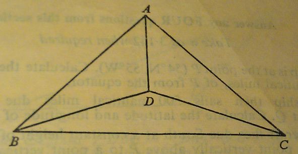
The diagram represents a roof-truss in which AB = AC = 8 m, BC = 11 m, BD = DC and ∠DBC = 20°.
Calculate
(a) the length BD,
(b) the angle ABC,
(c) the length AD.
- Draw the graph of
 for values of from -1 to +4, taking 2 cm as one unit on the x-axis and 1 cm as one unit on the y-axis. From your graph, find the range of values of for which the function
  is greater than 6.
Using the sane axes and scales, draw the graph of
 and write down the coordinates of the points of intersection of the two graphs.
if
 is the quadratic equation of which these coordinates are the roots, determine the values of
  and .
and .17 marks
- A particle starts from rest at a point A and moves along a straight line, coming to rest again at another point B. During the motion its velocity,
 metres per second, after time
  is given by
  .
.
Calculate:
(a) the time taken for the particle to reach B.
(b) the distance travelled during the first two seconds,
(c) the time taken for the particle to attain its maximum velocity,
(d) the maximum velocity attained,
(e) the maximum acceleration during the motion.
17 marks
Recent Comments