Archive
Maximum Adds per second for 1950s/early 1960s computers
Relative digital computer performance has been measured, since the mid-1960s, by timing how long it takes to execute one or more programs. Until the early 1990s Whetstone was widely used, and then SPEC brought things up to date.
Running the same program on multiple computers requires that it be written in a language that is available on those computers. Fortran, Cobol and Algol 60 started to spread at the start of the 1960s (there were 21 Algol 60 compilers were available in 1961), but it took a while for old habits to change, and for specific programs to be accepted as reasonable benchmarks.
One early performance comparison method involved calculating a sum of instruction timings, weighted by instruction frequency. The view of computers as calculating machines meant that the arithmetic instructions add/multiply/divide were often the focus of attention.
A calculation based on instructions assumes that timings do not vary with the value of the operand (which multiple and divide often do, and addition sometimes does), that instruction time can be measured independent of the time taken to load the values from memory (which is not possible for when one operand is always loaded from memory), and instruction frequency is representative of typical applications.
With regard to instruction timings, some manufacturers quoted an average, while others gave a range of values. One publication quotes arithmetic timings for specific numeric values. The “Data Processing Equipment Encyclopedia: Electronic Devices”, published in 1961 by Gille Associates, lists the characteristics of 104 computers, including the time taken to perform the arithmetic operations: addition 555555+555555, multiplication 555555*555555, and division 308641358025/555555. The results were mostly for fixed point, sometimes floating-point, or both, and once in double precision. In practice small numeric values dominate program execution. I suspect the publishers picked large values because customers think of computers as working on big/complicated problems.
The time taken to load a value from memory can be a significant percentage of execution time, which is why processor cache has such a big impact on performance. In the 1950s main memory was often the cache, with the rest of memory held on a rotating drum. Hardware specifications often gave arithmetic instruction timings for both excluded and included memory access cases.
The plot below shows the execution time of the Add instruction excluding/including memory access on the same computer for pre-1961 computers, with regression line of the form:  (grey line shows
  ; code+data):
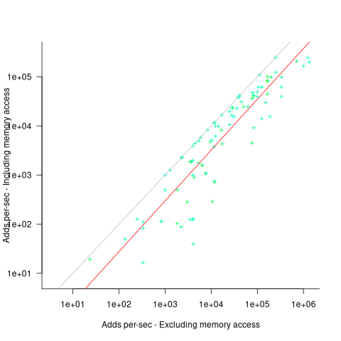
When memory access time is included in the Add instruction timing, the maximum rate of instructions per second decreases by approximately a factor of four, compared to when memory access time is excluded.
What was the frequency distribution of instructions executed by computers in the 1950s/1960s? I suspect it was a simplified form of today’s frequency distribution. Simplified in the sense of there being fewer variants of commonly used instructions and way fewer addressing modes.
Application domains were divided into scientific/engineering and commercial. One executed lots of float-point instructions, the other executed none. One did a lot of reading/writing of punched cards/magnetic tape, the other did hardly any. If we want to compare early the performance of cpus across the decades, methods that assume a significant amount of I/O have to be ignored, or the I/O component reverse engineered out.
Kenneth Knight, in his PhD thesis (no copy online), published the most detailed and extensive analysis, and data. Knight included an I/O component in his performance formula, but this was relatively small for scientific/engineering.
The table below lists the instruction weights for scientific/engineering applications published by Knight and Arbuckle, a Manager of Product Marketing at IBM:
Instruction or Operation Knight Arbuckle Floating Point Add/Sub 10% 9.5% Floating Point Multiply 6% 5.6% Floating Point Divide 2% 2.0% Fixed add/sub 10% Load/Store 28.5% Indexing 22.5% Conditional Branch 13.2% Miscellaneous 72% 18.7% |
Solomon published weights for the IBM 360 family. By focusing on a range of compatible computers the evaluation was not restricted to generic operations, and used timings from 60 different instructions.
The following analysis is based on data extracted from the 1955, 1961, and 1964 (which does not have a handy table of arithmetic instruction timings; thanks to Ed Thelen for converting the scanned images) surveys of domestic electronic digital computing systems published by the Ballistic Research Laboratory.
If the performance of computers from the 1950s/1960s is to be compared with performance in later decades, which computers from the 1950s/1960s should be included? Of the 228 computers listed in a January 1964 survey of the roughly 14k+ computing systems manufactured or operational, over 50% are bespoke, i.e., they are unique. The top 10 systems represent over 75% of manufactured systems; see table below (the IBM 604 was an electronic calculating punch, and is not listed):
   Quantity   SYSTEM           Cumulative percentage
   5,000+      IBM 1401                  36%
   2,500+      IBM 650                   54%
     693       IBM CPC                   59%
     490       LGP 30                    63%
     478       BURROUGHS B26O/B270/B280  66%
     400+      LIBRATROL 500             69%
     300+      BENDIX G-15               71%
     300       CONTROL DATA 160A         73%
     267       IBM 607                   75%
210 BURROUGHS E103/E101 77% |
When programming in machine code, developers put a lot of effort into keeping frequently used values in registers (developers can still sometimes do a better job than compilers), and overlapping memory access with other operations. The plot below shows the maximum number of add and multiply instructions per second that could be executed without accessing storage (code+data):
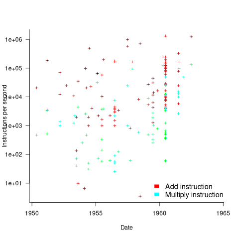
The systems capably of less than ten instructions per second are essentially early desktop calculators.
What percentage of Add instructions accessed memory? As far as I can tell, none of the performance comparison reports/papers address with this question. To be continued…
CPU power consumption and bit-similarity of input
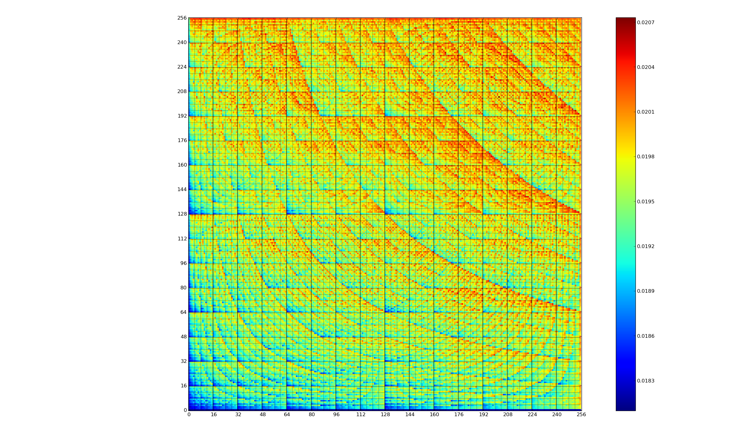
Changing the state of a digital circuit (i.e., changing its value from zero to one, or from one to zero) requires more electrical power than leaving its state unchanged. During program execution, the power consumed by each instruction depends on the value of its operand(s). The plot below, from an earlier post, shows how the power consumed by an 8-bit multiply instruction varies with the values of its two operands:
An increase in cpu power consumption produces an increase in its temperature. If the temperature gets too high, the cpu’s DVFS (dynamic voltage and frequency scaling) will slow down the processor to prevent it overheating.
When a calculation involves a huge number of values (e.g., an LLM size matrix multiply), how large an impact is variability of input values likely to have on the power consumed?
The 2022 paper: Understanding the Impact of Input Entropy on FPU, CPU, and GPU Power by S. Bhalachandra, B. Austin, S. Williams, and N. J. Wright, compared matrix multiple power consumption when all elements of the matrices had the same values (i.e., minimum entropy) and when all elements had different random values (i.e., maximum entropy).
The plot below shows the power consumed by an NVIDIA A100 Ampere GPU while multiplying two 16,384 by 16,384 matrices (performed 100 times). The GPU was power limited to 400W, so the random value performance was lower at 18.6 TFLOP/s, against 19.4 TFLOP/s for same values; (I don’t know why the startup times differ; code+data):
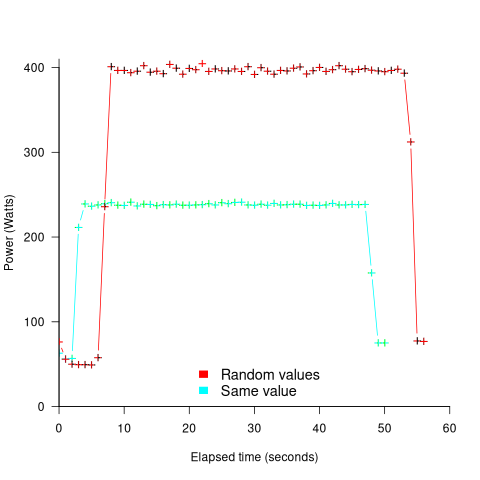
This 67% performance difference is more than an interesting factoid. Large computations are distributed over multiple GPUs, and the output from each GPU is sometimes feed as input to other GPUs. The flow of computations around a cluster of GPUs needs to be synchronised, and having compute time depend on the distribution of the input values makes life complicated.
Is it possible to organise a sequence of calculation to reduce the average power consumed?
The higher order bits of small integers are zero, but how many long calculations involve small integers? The bit pattern of floating-point values are more difficult to predict, but I’m sure there is a PhD thesis or two waiting to be written around this issue.
Distribution of add/multiply expression values
The implementation of scientific/engineering applications requires evaluating many expressions, and can involve billions of adds and multiplies (divides tend to be much less common).
Input values percolate through an application, as it is executed. What impact does the form of the expressions evaluated have on the shape of the output distribution; in particular: What is the distribution of the result of an expression involving many adds and multiplies?
The number of possible combinations of add/multiply grows rapidly with the number of operands (faster than the rate of growth of the Catalan numbers). For instance, given the four interchangeable variables: w, x, y, z, the following distinct expressions are possible: w+x+y+z, w*x+y+z, w*(x+y)+z, w*(x+y+z), w*x*y+z, w*x*(y+z), w*x*y*z, and w*x+y*z.
Obtaining an analytic solution seems very impractical. Perhaps it’s possible to obtain a good enough idea of the form of the distribution by sampling a subset of calculations, i.e., the output from plugging random values into a large enough sample of possible expressions.
What is needed is a method for generating random expressions containing a given number of operands, along with a random selection of add/multiply binary operators, then to evaluate these expressions with random values assigned to each operand.
The approach I used was to generate C code, and compile it, along with the support code needed for plugging in operand values (code+data).
A simple method of generating postfix expressions is to first generate operations for a stack machine, followed by mapping this to infix form to a postfix form.
The following awk generates code of the form (‘executing’ binary operators, o, right to left): o v o v v. The number of variables in an expression, and number of lines to generate, are given on the command line:
# Build right to left function addvar() { num_vars++ cur_vars++ expr="v " expr # choose variable later } function addoperator() { cur_vars-- expr="o " expr # choose operator later } function genexpr(total_vars) { cur_vars=2 num_vars=2 expr="v v" # Need two variables on stack while (num_vars <= total_vars) { if (cur_vars == 1) # Must push a variable addvar() else if (rand() > 0.2) # Seems to produce reasonable expressions addvar() else addoperator() } while (cur_vars > 1) # Add operators to use up operands addoperator() print expr } BEGIN { # NEXPR and VARS are command line options to awk if (NEXPR != "") num_expr=NEXPR else num_expr=10 for (e=1; e <=num_expr; e++) genexpr(VARS) } |
the following awk code maps each line of previously generated stack machine code to a C expression, wraps them in a function, and defines the appropriate variables.
function eval(tnum) { if ($tnum == "o") { printf("(") tnum=eval(tnum+1) #recurse for lhs if (rand() <= PLUSMUL) # default 0.5 printf("+") else printf("*") tnum=eval(tnum) #recurse for rhs printf(")") } else { tnum++ printf("v[%d]", numvars) numvars++ # C is zero based } return tnum } BEGIN { numexpr=0 print "expr_type R[], v[];" print "void eval_expr()" print "{" } { numvars=0 printf("R[%d] = ", numexpr) numexpr++ # C is zero based eval(1) printf(";\n") next } END { # print "return(NULL)" printf("}\n\n\n") printf("#define NUMVARS %d\n", numvars) printf("#define NUMEXPR %d\n", numexpr) printf("expr_type R[NUMEXPR], v[NUMVARS];\n") } |
The following is an example of a generated expression containing 100 operands (the array v is filled with random values):
R[0] = ((((((((((((((((((((((((((((((((((((((((((((((((( ((((((((((((((((((((((((v[0]*v[1])*v[2])+(v[3]*(((v[4]* v[5])*(v[6]+v[7]))+v[8])))*v[9])+v[10])*v[11])*(v[12]* v[13]))+v[14])+(v[15]*(v[16]*v[17])))*v[18])+v[19])+v[20])* v[21])*v[22])+(v[23]*v[24]))+(v[25]*v[26]))*(v[27]+v[28]))* v[29])*v[30])+(v[31]*v[32]))+v[33])*(v[34]*v[35]))*(((v[36]+ v[37])*v[38])*v[39]))+v[40])*v[41])*v[42])+v[43])+ v[44])*(v[45]*v[46]))*v[47])+v[48])*v[49])+v[50])+(v[51]* v[52]))+v[53])+(v[54]*v[55]))*v[56])*v[57])+v[58])+(v[59]* v[60]))*v[61])+(v[62]+v[63]))*v[64])+(v[65]+v[66]))+v[67])* v[68])*v[69])+v[70])*(v[71]*(v[72]*v[73])))*v[74])+v[75])+ v[76])+v[77])+v[78])+v[79])+v[80])+v[81])+((v[82]*v[83])+ v[84]))*v[85])+v[86])*v[87])+v[88])+v[89])*(v[90]+v[91])) v[92])*v[93])*v[94])+v[95])*v[96])*v[97])+v[98])+v[99])*v[100]); |
The result of each generated expression is collected in an array, i.e., R[0], R[1], R[2], etc.
How many expressions are enough to be a representative sample of the vast number that are possible? I picked 250. My concern was the C compilers code generator (I used gcc); the greater the number of expressions, the greater the chance of encountering a compiler bug.
How many times should each expression be evaluated using a different random selection of operand values? I picked 10,000 because it was a big number that did not slow my iterative trial-and-error tinkering.
The values of the operands were randomly drawn from a uniform distribution between -1 and 1.
What did I learn?
- Varying the number of operands in the expression, from 25 to 200, had little impact on the distribution of calculated values.
- Varying the form of the expression tree, from wide to deep, had little impact on the distribution of calculated values.
- Varying the relative percentage of add/multiply operators had a noticeable impact on the distribution of calculated values. The plot below shows the number of expressions (binned by rounding the absolute value to three digits) having a given value (the power law exponents fitted over the range 0 to 1 are: -0.86, -0.61, -0.36; code+data):
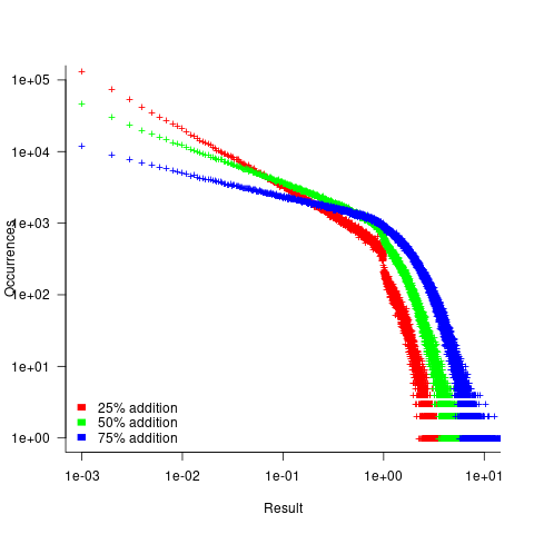
A rationale for the change in the slopes, for expressions containing different percentages of add/multiply, can be found in an earlier post looking at the distribution of many additions (the Irwin-Hall distribution, which tends to a Normal distribution), and many multiplications (integer power of a log).
- The result of many additions is to produce values that increase with the number of additions, and spread out (i.e., increasing variance).
- The result of many multiplications is to produce values that become smaller with the number of multiplications, and become less spread out.
Which recent application spends a huge amount of time adding/multiplying values in the range -1 to 1?
Large language models. Yes, under the hood they are all linear algebra; adding and multiplying large matrices.
LLM expressions are often evaluated using a half-precision floating-point type. In this 16-bit type, the exponent is biased towards supporting very small values, at the expense of larger values not being representable. While operations on a 10-bit significand will experience lots of quantization error, I suspect that the behavior seen above not noticeable change.
Recent Comments