The Shape of Code

Some programs perform one basic task, e.g., analyse input to calculate some quantity. These programs often take a set of input values and produce some output.

If a program contains a single coding mistake and the probability of producing incorrect output, for one set of inputs, is , the probability of the ‘th output being incorrect is: 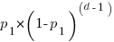. This is a geometric distribution (an exponential distribution is a good enough approximation). The value can be thought of as the distance between incorrect outputs, measured in the number of distinct inputs correctly processed.

If the program contains a second, different, coding mistake, whose probability of producing incorrect output, for a given input, is , the probability of incorrect output after inputs is now: . And so on for each distinct coding mistake.

The value of is driven by the likelihood that the input values cause the program’s flow of control to reach the code containing the coding mistake, and then for the execution of the coding mistake to produce a value that percolates through the executed code to produce an incorrect output value. It might be said that users cause faults by providing the necessary input values.

Each in the expression is created by the distinct coding mistakes, .

In practice the number of distinct coding mistakes, , is unknown, and a single probability is assigned to incorrect output: , giving: 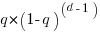(the substitution is a good enough approximation because the are very small).

How accurate is this model in practice?

The analysis below uses data from my top, must read, paper on software fault analysis and a recent study of LLM driven N-version programming.

The N-Version Programming with Coding Agents tested 1-million inputs/outputs, and 14 of the programs in the published results contained 421 incorrect outputs (data kindly provided by Javier Ron). Before discussing the same incorrect counts, does the ‘distance’ between incorrect outputs have an exponential distribution?

This question can be answered using an exponential Q-Q plot (values predicted by theory on the x-axis, actual values on the y-axis). The plot below shows the actual values (blue/green) and a fitted regression line (data from running the claude_code__m_claude-haiku-4.5__l_rust__run000 generated code; code+data):

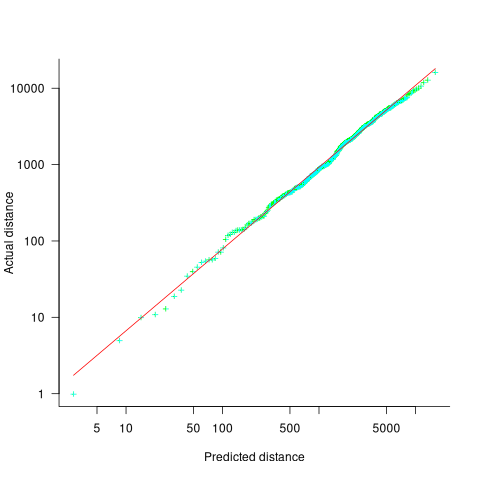
If the data had an exponential distribution the exponent of a fitted power law would be exactly 1. However, the fitted exponent is 1.07, and is statistically significant (for the sample size and standard error of the fit).

The above analysis assumes that the probability of incorrect output, , is constant. In practice varies across different input values, but over very many inputs is assumed to be clustered around an unchanging average value. It is possible that the input values are divided into two clusters whose incorrect output probabilities are and , i.e., a mixture of two exponentials. The worst case scenario is a mixture of umpteen exponentials.

Fitting the distance data to a mixture of two exponentials gives: (code+data). This corresponds to 10% of the input having an average distance between incorrect output of 482, and 90% having a distance of 2,735 (average 2,482), i.e., one cluster of input values is a lot more likely to produce incorrect output than the other cluster. In the published data the average distance is 2,385.

The specification used for the N-version studies came from a study by Nagel and Skrivan who tracked down each of the coding mistakes in the programs tested. They found that around 80% of incorrect outputs were caused by the same coding mistake, and 16% by a second coding mistake (see figure 4.3.7.1-1; an analysis of the Knight & Leveson coding mistakes). Once these two coding mistakes were fixed, other coding mistakes caused incorrect output.

For the LLM generated code, 14 out of the 59 programs had 421 incorrect outputs. Did the LLMs all generate code containing the same coding mistake? I have yet to track down any of the coding mistakes, or get an LLM to do it for me. Once a few coding mistakes have been fixed, ‘allowing’ other coding mistakes to produce incorrect output, will partially correct LLM generated programs stop having correlated failures?

How much does the number of incorrect output change when a different set of random inputs are used?

The random seed used in the published results is: 42. I replicated this output for all 56 programs (it takes around 8.5 hours on my system), and then ran the 1-million inputs on just four programs using the seeds: 101, 20101, 321, 789, and 6000 (which each took around 1-hour). The table below shows the number of incorrect outputs for the various seeds (each numeric column corresponds to a different seed):

        Generation information                 Number of incorrect outputs
claude_code__m_claude-haiku-4.5__l_rust      421   432   374  404  424   452
codex__m_gpt-5.1-codex__l_pascal             421   431   372  402  424   451
claude_code__m_claude-sonnet-4.6__l_pascal  1222  1224  1214 1237 1207  1282
codex__m_gpt-5.4-mini__l_python            10052 10063 10181 9944 9963 10122

Two (claude_code__m_claude-haiku-4.5__l_rust and codex__m_gpt-5.1-codex__l_pascal) of the 14 programs that had the same number of incorrect outputs with seed 42, had slightly different number of incorrect outputs with other seeds. This suggests that their coding mistakes are slightly different.

All the generated programs had some deviation from the pure single exponential model discussed above.

This simple model for ‘distance’ between incorrect outputs is a good fit to reality because the program performs one basic function and is relatively short (around 500 lines). Larger programs supporting a selection of functionality are going to require much more complicated models.