Archive
Specification based programming
The use of LLM to write software has focused on integrating them within existing practices, i.e., using LLMs as very fancy auto-completers for chunks of code or functionality. This use is programming by conversation, or less politely, programming by stream of thought. The term vibe-coding creates an illusion of trendiness; after all, software engineering is a hedonistic activity.
With vibe-code on top of vibe-code on top of vibe-code, refactoring becomes a complete rewrite, at least in theory. A rewrite assumes that it’s possible to extract a specification that is complete and accurate enough to recreate the software. A lot of software has a short lifetime, so a major rewrite may never be needed. However, for software that is expected to have a long life, management are going to want a more controlled/structured/repeatable approach.
LLMs’ ability to write software is now good enough to support a more controlled/structured/repeatable approach: Programming by specification. That is a specification of the desired behavior is given to one or more LLMs, which use it to generate the appropriate software.
The human input to the program creation process is via the specification.
Features are changed/added/removed by updating the specification. Bugs are fixed by updating the specification. If there are mistakes in the generated code, the specification has to work around them, in the same way that compiler bugs have to be worked around.
Business logic can be expressed as a specification, which is how application domain experts, who are not programmers, are able to create minimal viable products using LLMs.
How might a specification be created?
Agile has taught the lesson that software creation is an iterative process. Requiring a complete specification before coding starts is the stuff of armchair project managers.
One possible specification iteration process starts with a basic outline specification of what is required, and is followed by the following cycle:
- Using the current specification, developer+LLM produces code. Perhaps particular functionality is implemented, or the work continues for some amount of time, or etc,
- the transcript of the LLM conversation is used to create an updated specification of the code that exists when work stopped. Conversations involving code that came and went is not part of the updated specification, although logging it for future reference costs little,
- a new version of all the software covered by the updated specification is generated. This can be tested using existing tests and also by differential testing using multiple implementations created from the same specification (a recent paper generated five implementations in different languages),
- if more functionality is needed, go to step 1.
Specifications share many characteristics with source code. They can be split up and organized into modules/packages/components/phases, as was done for this LLM generated C compiler.
LLM generated code is more verbose than human generated code, just like the machine code generated by early compilers.
Open source projects could soon just be making the specification available. Why ship the source code generated from a specification, projects don’t ship the assembler code generated by compilers, they ship the original source code. However, given the current reliability of LLM source code generation, they are benefits to making the generated source of at least one implementation available (as a kind of checksum).
Reduced implementation costs, using LLMs, make it possible to create programs containing more functionality (Jevrons paradox in action). This in turned leads to specifications becoming larger, complicated and poorly organized, just like source code.
English usage is full of ambiguities. This ambiguity can be reduced by using a controlled language. If specification programming becomes popular, it’s easy to imagine the invention of controlled languages becoming as popular as the invention of programming languages. In 1957, there were compilers for at least 28 programming languages.
Specification based programming is a continuation of the trend of computers handling more of the details involved in program creation, with the program creation process requiring less and less knowledge about computers. Increasing amounts of computer time are spent to reduce or eliminate developer time.
Programming has evolved from physically connecting subsystems by cables to specify the flow of bits in a punch card computer, to a sequence of machine code instructions executed by a stored-program computer, then high-level programming languages reducing the need to know lots of details about the underlying cpu (details that remain include: number of bits in the integer types and type compatibility rules).
Specification based programming requires discipline, and I don’t expect it to be popular. I expect multiple LLM-derived project disasters need to occur before there are any significant changes to the current LLM approaches to software development.
Sample size needed to compare performance of two languages
A humungous organization wants to minimise one or more of: program development time/cost, coding mistakes made, maintenance time/cost, and have decided to use either of the existing languages X or Y.
To make an informed decision, it is necessary to collect the required data on time/cost/mistakes by monitoring the development process, and recording the appropriate information.
The variability of developer performance, and language/problem interaction means that it is necessary to monitor multiple development teams and multiple language/problem pairs, using statistical techniques to detect any language driven implementation performance differences.
How many development teams need to be monitored to reliably detect a performance difference driven by language used, given the variability of the major factors involved in the process?
If we assume that implementation times, for the same program, have a normal distribution (it might lean towards lognormal, but the maths is horrible), then there is a known formula. Three values need to be specified, and plug into this formula: the statistical significance (i.e., the probability of detecting an effect when none is present, say 5%), the statistical power (i.e., the probability of detecting that an effect is present, say 80%), and Cohen’s d; for an overview see section 10.2.
Cohen’s d is the ratio 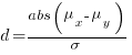 , where
  and
and  is the mean value of the quantity being measured for the programs written in the respective languages, and
  is the pooled standard deviation.
Say the mean time to implement a program is , what is a good estimate for the pooled standard deviation, , of the implementation times?
Having 66% of teams delivering within a factor of two of the mean delivery time is consistent with variation in LOC for the same program and estimation accuracy, and if anything sound slow (to me).
Rewriting the Cohen’s d ratio: 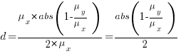
If the implementation time when using language X is half that of using Y, we get 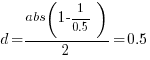 . Plugging the three values into the
 pwr.t.test function, in R’s pwr package, we get:
> library("pwr")
> pwr.t.test(d=0.5, sig.level=0.05, power=0.8)

     Two-sample t test power calculation

              n = 63.76561
              d = 0.5
      sig.level = 0.05
          power = 0.8
    alternative = two.sided

NOTE: n is number in *each* group |
In other words, data from 64 teams using language X and 64 teams using language Y is needed to reliably detect (at the chosen level of significance and power) whether there is a difference in the mean performance (of whatever was measured) when implementing the same project.
The plot below shows sample size required for a t-test testing for a difference between two means, for a range of X/Y mean performance ratios, with red line showing the commonly used values (listed above) and other colors showing sample sizes for more relaxed acceptance bounds (code):
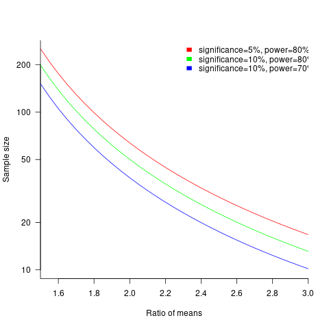
Unless the performance difference between languages is very large (e.g., a factor of three) the required sample size is going to push measurement costs into many tens of millions (£1 million per team, to develop a realistic application, multiplied by two and then multiplied by sample size).
For small programs solving certain kinds of problems, a factor of three, or more, performance difference between languages is not unusual (e.g., me using R for this post, versus using Python). As programs grow, the mundane code becomes more and more dominant, with the special case language performance gains playing an outsized role in story telling.
There have been studies comparing pairs of languages. Unfortunately, most have involved students implementing short problems, one attempted to measure the impact of programming language on coding competition performance (and gets very confused), the largest study I know of compared Fortran and Ada implementations of a satellite ground station support system.
The performance difference detected may be due to the particular problem implemented. The language/problem performance correlation can be solved by implementing a wide range of problems (using 64 teams per language).
A statistically meaningful comparison of the implementation costs of language pairs will take many years and cost many millions. This question is unlikely to every be answered. Move on.
My view is that, at least for the widely used languages, the implementation/maintenance performance issues are primarily driven by the ecosystem, rather than the language.
Criteria for increased productivity investment
You have a resource of  person days to implement a project, and believe it is worth investing some of these days,
  , to improve team productivity (perhaps with training, or tooling). What is the optimal amount of resource to allocate to maximise the total project work performed (i.e., excluding the performance productivity work)?
Without any productivity improvement, the total amount of project work is:
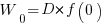 , where
  is the starting team productivity function, f, i.e., with zero investment.
After investing person days to increase team productivity, the total amount of project work is now:
 , where
  is the team productivity function, f, after the investment .
To find the value of that maximises  , we differentiate with respect to , and solve for the result being zero:
 , where
  is the differential of the yet to be selected function
  .
.
Rearranging this equation, we get:
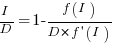
We can plug in various productivity functions, , to find the optimal value of .
For a linear relationship, i.e.,  , where
  is the unit productivity improvement constant for a particular kind of training/tool, the above expression becomes:
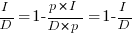
Rearranging, we get:  , or
, or  .
.
The surprising (at least to me) result that the optimal investment is half the available days.
It is only worthwhile making this investment if it increases the total amount of project work. That is, we require:  .
.
For the linear improvement case, this requirement becomes:
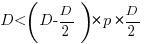 , or
, or 
This is the optimal case, but what if the only improvement options available are not able to sustain a linear improvement rate of at least  ? How many days should be invested in this situation?
A smaller investment,  , is only worthwhile when:
 , where
  , and
, and  .
.
Substituting gives:  , which simplifies to:
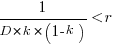
The blue/green line plot below shows the minimum value of  for
for  (and
(and  , increasing moves the line down), with the red line showing the optimal value
  . The optimal value of
  is at the point where has its minimum worthwhile value (the derivative of
  is
is  ; code):
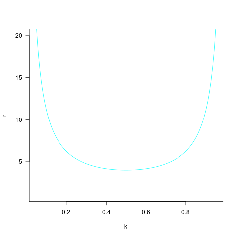
This shows that it is never worthwhile making an investment when:  , and that when it is always worthwhile investing , with any other value either wasting time or not extracting all the available benefits.
In practice, an investment may be subject to diminishing returns.
When the rate of improvement increases as the square-root of the number of days invested, i.e.,  , the optimal investment, and requirement on unit rate are as follows:
only invest:  , when:
If the rate of improvement with investment has the form:  , the respective equations are:
only invest:  , when:
 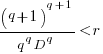 . The minimal worthwhile value of always occurs at the optimal investment amount.
When the rate of improvement is logarithmic in the number of days invested, i.e.,  , the optimal investment, and requirement on unit rate are as follows:
only invest: 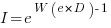 , where
  is the Lambert W function, when: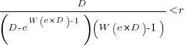
These expressions can be simplified using the approximation  , giving:
only invest: 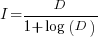 , when:
In practice, after improving rapidly, further investment on improving productivity often produces minor gains, i.e., the productivity rate plateaus. This pattern of rate change is often modelled using a logistic equation, e.g.,  .
.
However, following the process used above for this logistic equation produces an equation for , 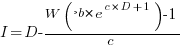 , that does not have any solutions when
  and are positive.
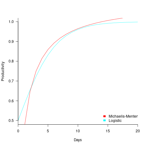
The problem is that the derivative goes to zero too quickly. The Michaelis-Menten equation,  , has an asymptotic limit whose derivative goes to zero sufficiently slowly that a solution is available.
only invest:  , when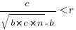
The plot below shows example Michaelis-Menten and Logistic equations whose coefficients have been chosen to produce similar plots over the range displayed (code):
These equations are all well and good. The very tough problem of estimating the value of the coefficients is left to the reader.
This question has probably been answered before. But I have not seen it written down anywhere. References welcome.
Analysis of when refactoring becomes cost-effective
In a cost/benefit analysis of deciding when to refactor code, which variables are needed to calculate a good enough result?
This analysis compares the excess time-code of future work against the time-cost of refactoring the code. Refactoring is cost-effective when the reduction in future work time is less than the time spent refactoring. The analysis finds a relationship between work/refactoring time-costs and number of future coding sessions.
Linear, or supra-linear case
Let’s assume that the time needed to write new code grows at a linear, or supra-linear rate, as the amount of code increases ( ):
):
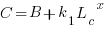
where:  is the base time for writing new code on a freshly refactored code base,
  is the number of lines of code that have been written since the last refactoring, and
  and
and  are constants to be decided.
The total time spent writing code over  sessions is:
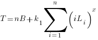
If the same number of new lines is added in every coding session,  , and is an integer constant, then the sum has a known closed form, e.g.:
x=1, 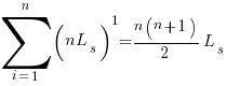 ; x=2,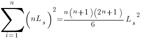
Let’s assume that the time taken to refactor the code written after sessions is:
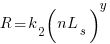
where:  and
and  are constants to be decided.
The reason for refactoring is to reduce the time-cost of subsequent work; if there are no subsequent coding sessions, there is no economic reason to refactor the code. If we assume that after refactoring, the time taken to write new code is reduced to the base cost, , and that we believe that coding will continue at the same rate for at least another sessions, then refactoring existing code after sessions is cost-effective when:
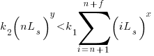
assuming that is much smaller than , setting  , and rearranging we get:
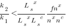
after rearranging we obtain a lower limit on the number of future coding sessions, , that must be completed for refactoring to be cost-effective after session ::

It is expected that  ; the contribution of code size, at the end of every session, in the calculation of
  and
and  is equal (i.e.,
 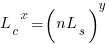 ), and the overhead of adding new code is very unlikely to be less than refactoring all the newly written code.
With  , must be close to zero; otherwise, the likely relatively large value of (e.g., 100+) would produce surprisingly high values of .
Sublinear case
What if the time overhead of writing new code grows at a sublinear rate, as the amount of code increases?
Various attributes have been found to strongly correlate with the  of lines of code. In this case, the expressions for and become:

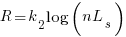
and the cost/benefit relationship becomes:
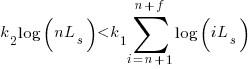
applying Stirling’s approximation and simplifying (see Exact equations for sums at end of post for details) we get:

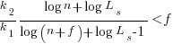
applying the series expansion (for  ):
): 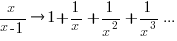 , we get
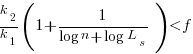
Discussion
What does this analysis of the cost/benefit relationship show that was not obvious (i.e., the relationship  is obviously true)?
What the analysis shows is that when real-world values are plugged into the full equations, all but two factors have a relatively small impact on the result.
A factor not included in the analysis is that source code has a half-life (i.e., code is deleted during development), and the amount of code existing after sessions is likely to be less than the  used in the analysis (see Agile analysis).
As a project nears completion, the likelihood of there being more coding sessions decreases; there is also the every present possibility that the project is shutdown.
The values of and encode information on the skill of the developer, the difficulty of writing code in the application domain, and other factors.
Exact equations for sums
The equations for the exact sums, for  , are:
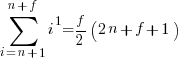


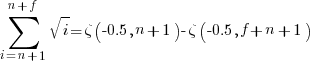 , where
  is the Hurwitz zeta function.
Sum of a log series: 
using Stirling’s approximation we get

simplifying

and assuming that is much smaller than gives

Update
The analysis above assumes that the time contribution of the base rate, , is independent of the changes,  . The following analysis combines these two contributions into a single rate:
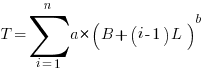
where:  ,
,  , , and are positive constants, with
  , and
, and  .
.
The following is a very good approximation to this sum (thanks to Grok 4.1 beta; chat script):
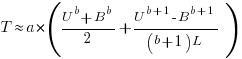
where: 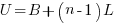
Cost-effectiveness decision for fixing a known coding mistake
If a mistake is spotted in the source code of a shipping software system, is it more cost-effective to fix the mistake, or to wait for a customer to report a fault whose root cause turns out to be that particular coding mistake?
The naive answer is don’t wait for a customer fault report, based on the following simplistic argument:  .
.
where:  is the cost of fixing the mistake in the code (including testing etc), and
  is the cost of finding the mistake in the code based on a customer fault report (i.e., the sum on the right is the total cost of fixing a fault reported by a customer).
If the mistake is spotted in the code for ‘free’, then  , e.g., a developer reading the code for another reason, or flagged by a static analysis tool.
This answer is naive because it fails to take into account the possibility that the code containing the mistake is deleted/modified before any customers experience a fault caused by the mistake; let  be the likelihood that the coding mistake ceases to exist in the next unit of time.
The more often the software is used, the more likely a fault experience based on the coding mistake occurs; let  be the likelihood that a fault is reported in the next time unit.
A more realistic analysis takes into account both the likelihood of the coding mistake disappearing and a corresponding fault being reported, modifying the relationship to: 
Software systems are eventually retired from service; the likelihood that the software is maintained during the next unit of time,  , is slightly less than one.
Giving the relationship: 
which simplifies to: 
What is the likely range of values for the ratio:  ?
?
I have no find/fix cost data, although detailed total time is available, i.e., find+fix time (with time probably being a good proxy for cost). My personal experience of find often taking a lot longer than fix probably suffers from survival of memorable cases; I can think of cases where the opposite was true.
The two values in the ratio  are likely to change as a system evolves, e.g., high code turnover during early releases that slows as the system matures. The value of should decrease over time, but increase with a large influx of new users.
A study by Penta, Cerulo and Aversano investigated the lifetime of coding mistakes (detected by several tools), tracking them over three years from creation to possible removal (either fixed because of a fault report, or simply a change to the code).
Of the 2,388 coding mistakes detected in code developed over 3-years, 41 were removed as reported faults and 416 disappeared through changes to the code: 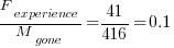
The plot below shows the survival curve for memory related coding mistakes detected in Samba, based on reported faults (red) and all other changes to the code (blue/green, code+data):
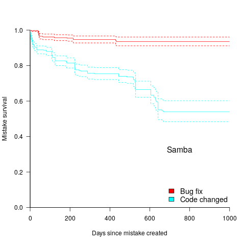
Coding mistakes are obviously being removed much more rapidly due to changes to the source, compared to customer fault reports.
For it to be cost-effective to fix coding mistakes in Samba, flagged by the tools used in this study ( is essentially one), requires:  .
.
Meeting this requirement does not look that implausible to me, but obviously data is needed.
Software engineering research problems having worthwhile benefits
Which software engineering research problems are likely to yield good-enough solutions that provide worthwhile benefits to professional software developers?
I can think of two (hopefully there are more):
- what is the lifecycle of software? For instance, the expected time-span of the active use of its various components, and the evolution of its dependency ecosystem,
- a model of the main processes involved in a software development project.
Solving problems requires data, and I think it is practical to collect the data needed to solve these two problems; here is some: application lifetime data, and detailed project data (a lot more is needed).
Once a good-enough solution is available, its practical application needs to provide a worthwhile benefit to the customer (when I was in the optimizing compiler business, I found that many customers were not interested in more compact code unless the executable was at least a 10% smaller; this was the era of computer memory often measured in kilobytes).
Investment decisions require information about what is likely to happen in the future, and an understanding of common software lifecycles is needed. The fact that most source code has a brief existence (a few years) and is rarely modified by somebody other than the original author, has obvious implications for investment decisions intended to reduce future maintenance costs.
Running a software development project requires an understanding of the processes involved. This knowledge is currently acquired by working on projects managed by people who have successfully done it before. A good-enough model is not going to replace the need for previous experience, some amount of experience is always going to be needed, but it will provide an effective way of understanding what is going on. There are probably lots of different good-enough ways of running a project, and I’m not expecting there to be a one-true-way of optimally running a project.
Perhaps the defining characteristic of the solution to both of these problems is lots of replication data.
Applications are developed in many ecosystems, and there is likely to be variations between the lifecycles that occur in different ecosystems. Researchers tend to focus on Github because it is easily accessible, which is no good when replications from many ecosystems are needed (an analysis of Github source lifetime has been done).
Projects come in various shapes and sizes, and a good-enough model needs to handle all the combinations that regularly occur. Project level data is not really present on Github, so researchers need to get out from behind their computers and visit real companies.
Given the payback time-frame for software engineering research, there are problems which are not cost-effective to attempt to answer. Suggestions for other software engineering problems likely to be worthwhile trying to solve welcome.
Recent Comments