Archive
Criteria for increased productivity investment
You have a resource of  person days to implement a project, and believe it is worth investing some of these days,
  , to improve team productivity (perhaps with training, or tooling). What is the optimal amount of resource to allocate to maximise the total project work performed (i.e., excluding the performance productivity work)?
Without any productivity improvement, the total amount of project work is:
") , where
, where ") is the starting team productivity function, f, i.e., with zero investment.
is the starting team productivity function, f, i.e., with zero investment.
After investing person days to increase team productivity, the total amount of project work is now:
*f(I)") , where
, where ") is the team productivity function, f, after the investment .
is the team productivity function, f, after the investment .
To find the value of that maximises  , we differentiate with respect to , and solve for the result being zero:
*f prime(I)-f(I) =0") , where
, where ") is the differential of the yet to be selected function
is the differential of the yet to be selected function  .
.
Rearranging this equation, we get:
}/{D*f prime(I)}")
We can plug in various productivity functions, , to find the optimal value of .
For a linear relationship, i.e., =p*I*f(0)") , where
, where  is the unit productivity improvement constant for a particular kind of training/tool, the above expression becomes:

Rearranging, we get:  , or
, or  .
.
The surprising (at least to me) result that the optimal investment is half the available days.
It is only worthwhile making this investment if it increases the total amount of project work. That is, we require:  < (D-I)*f(I)") .
.
For the linear improvement case, this requirement becomes:
*p*{D/2}") , or
, or 
This is the optimal case, but what if the only improvement options available are not able to sustain a linear improvement rate of at least  ? How many days should be invested in this situation?
A smaller investment,  , is only worthwhile when:
 < (D-s)*f(s)") , where
, where  , and
, and  .
.
Substituting gives:  < (D-k*D)*r*k*D*f(0)") , which simplifies to:
, which simplifies to:
} < r")
The blue/green line plot below shows the minimum value of  for
for  (and
(and  , increasing moves the line down), with the red line showing the optimal value
  . The optimal value of
  is at the point where has its minimum worthwhile value (the derivative of
 }") is
is ^2}") ; code):
; code):
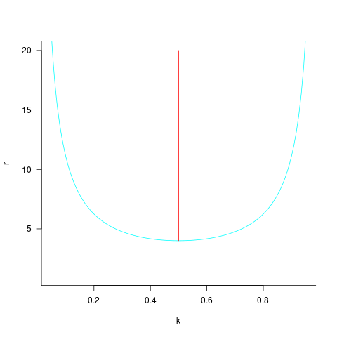
This shows that it is never worthwhile making an investment when:  , and that when it is always worthwhile investing , with any other value either wasting time or not extracting all the available benefits.
In practice, an investment may be subject to diminishing returns.
When the rate of improvement increases as the square-root of the number of days invested, i.e., =p*sqrt{I}*f(0)") , the optimal investment, and requirement on unit rate are as follows:
, the optimal investment, and requirement on unit rate are as follows:
only invest:  , when:
If the rate of improvement with investment has the form:  , the respective equations are:
only invest:  , when:
 ^{q+1}/{q^q D^q} < r") . The minimal worthwhile value of always occurs at the optimal investment amount.
. The minimal worthwhile value of always occurs at the optimal investment amount.
When the rate of improvement is logarithmic in the number of days invested, i.e., =p*log{I}*f(0)") , the optimal investment, and requirement on unit rate are as follows:
, the optimal investment, and requirement on unit rate are as follows:
only invest: -1}") , where
, where  is the Lambert W function, when:
 -1})(W(e*D)-1)} < r")
These expressions can be simplified using the approximation  approx log(x)-log(log(x))") , giving:
, giving:
only invest: }") , when:
, when: }/{(2+log(D))(log(D)-log(1+log(D)))} < r")
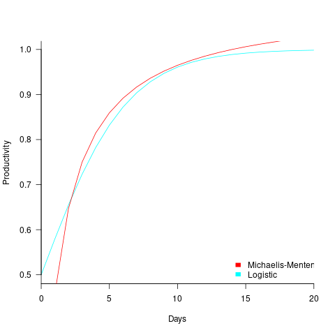
In practice, after improving rapidly, further investment on improving productivity often produces minor gains, i.e., the productivity rate plateaus. This pattern of rate change is often modelled using a logistic equation, e.g.,  .
.
However, following the process used above for this logistic equation produces an equation for , -1}/c") , that does not have any solutions when
, that does not have any solutions when  and are positive.
The problem is that the derivative goes to zero too quickly. The Michaelis-Menten equation,  , has an asymptotic limit whose derivative goes to zero sufficiently slowly that a solution is available.
only invest:  , when
The plot below shows example Michaelis-Menten and Logistic equations whose coefficients have been chosen to produce similar plots over the range displayed (code):
These equations are all well and good. The very tough problem of estimating the value of the coefficients is left to the reader.
This question has probably been answered before. But I have not seen it written down anywhere. References welcome.
Recent Comments