Archive
Employment in the software business: we know nothing
Tens of millions of people get paid to work on the creation and maintenance of software systems, by companies employing thousands of developers to those employing a single developer (in the UK there are almost 300K registered software companies; 5% of registered companies).
This huge ecosystem is almost completely ignored by the software engineering research community. Academics in computing/software are more interested in technical issue, and industry is an ecosystem they rarely interact with (some claim that student employment keeps them in contact with industry).
There are researchers in business and economics departments who study employment, e.g., careers, organization of workers and companies. The scientific study of work started at the beginning of the 1900s, originally focused on the manufacturing and included office work as that grew to employ a significant percentage of the workforce. Until recently, the percentage of the workforce employed to create/maintain software was not large enough to attract the attention of these researchers, and even now it’s often lumped together with other jobs that mostly involve some form of intellectual activity.
Employee related issues of interest to those involved in managing work on software systems are heavily influenced by the characteristics of the business ecosystem in which they work. The software driven business ecosystems are continually changing, with companies growing, merging and going bust as new markets emerge, grow, saturate, and sometime disappear. This constant change creates employment uncertainty, and lots of opportunities for competent people (creating a staff retention problem). For more stable industries, it’s possible for researchers to model employee start/promotion/leaving transitions using Markov models (example of ChatGPT 1o-preview solving a recurrence model of the staffing relationships in a 3-level employment hierarchy). The book “Stochastic Models for Social Processes” by D. J. Bartholomew gives a practical introduction to the use of Markov models for this kind of analysis.
The evolution and constant introduction of new technologies can make it difficult to find people with the appropriate skills. Companies may tune the wording of job adverts to give the impress of using ‘modern’ technologies, or post fake job adverts (to increase their attractiveness and suggest a feeling of growth), and people tune their CV to appeal to employers (some out right lie about their skills; many managers have told me that around 90% of applicants don’t have the primary skill sought by the employer). Well paid jobs can attract lots of applicants, filtering/interviewing can be an expensive process (not least because the same job title can denote different seniority in different companies). Matching CVs to job requirements sounds like the perfect use case for LLMs. I suspect that LLM tuning of CVs/adverts will just increase costs/uncertainty.
The constant churn of technologies forces employees to make decisions about whether to happily spend many years being well paid to become an expert in a niche with decreasing industry demand, or to invest in starting again as a non-expert doing something new (and initially less well paid).
What is the best to organize engineering employees at a company-wide scale? Matrix management was once the standard answer, but these days, scaled agile is a fashionable answer. An evidence-based answer will have to wait until the lawyers in a large organization allow somebody with the necessary skills access to the appropriate data.
With the contents of job sites being scraped, along with LinkedIn, I’m optimistic that some meaningful employment data will slowly become available. Will the analysis of this data uncover patterns of practical use (other than interesting blog posts) to employers/employees? We will have to wait and see.
C compiler conformance testing: with ChatGPT assistance
How can developers check that a compiler correctly implements all the behavior requirements contained in the corresponding language specification?
An obvious approach is to write lots of test cases for each distinct behavior; such a collection of tests is known as a validation suite, when used by a standard’s organization to test compilers/OS interfaces/etc. The extent to which a compiler’s behavior, when fed these tests, matches that listed in the language specification is a measure of its conformance.
In a world of many compilers with significant differences in behavior (i.e., pre-Open source), it makes economic sense for governments to sponsor the creation of validation suites, and/or companies to offer such suites commercially (mainly for C and C++). The spread of Open source compilers decimated compiler diversity, and compiler validation is fading into history.
New features continue to be added to Cobol, Fortran, C, and C++ by their respective ISO Standard’s committee. If governments are no longer funding updates to validation suites and the cost of commercial suites is too high for non-vendors (my experience is that compiler vendors find them to be cost-effective), how can developers check that a compiler conforms to the behavior specified by the Standard?
How much effort is required to create some minimal set of compiler conformance tests?
C is the language whose requirements I am most familiar with. The C Standard specifies that a conforming compiler issue a diagnostic for a violation of a requirement appearing in a Constraint clause, e.g., “For addition, either both operands shall have arithmetic type, or …”
There are 80 such clauses, containing around 530 non-blank lines, in N3301, the June 2024 draft. Let’s say 300+ distinct requirements, requiring a minimum of one test each. Somebody very familiar with the C Standard might take, say, 10 minutes per test, which is 3,000 minutes, or 50 hours, or 6.7 days; somebody slightly less familiar might take, say, at least an hour, which is 300+ hours, or 40+ days.
Lots of developers are using LLMs to generate source code from a description of what is needed. Given Constraint requirements in the C Standard, can an LLM generate tests that do a good enough job checking a compiler’s conformance to the C Standard?
Simply feeding the 157 pages from the Language chapter of the C Standard into an LLM, and asking it to generate tests for each Constraint requirement does not seem practical with the current state of the art; I’m happy to be proved wrong. A more focused approach might produce the desired tests.
Negative tests are likely to be the most challenging for an LLM to generate, because most publicly available source deals with positive cases, i.e., it is syntactically/semantically correct. The wording of Constraints sometimes specifies what usage is not permitted (e.g., clause 6.4.5.3 “A floating suffix df, dd, dl, DF, DD, or DL shall not be used in a hexadecimal floating literal.”), other times specifies what usage is permitted (e.g., clause 6.5.3.4 “The first operand of the . operator shall have an atomic, qualified, or unqualified structure or union type, and the second operand shall name a member of that type.”), or simply specifies a requirement (e.g., clause 6.7.3.2 “A member declaration that does not declare an anonymous structure or anonymous union shall contain a member declarator list.”).
I took the text from the 80 Constraint clauses, removed footnote numbers and rejoined words split at line-breaks. The plan was to prefix the text of each Constraint with instructions on the code requires. After some experimentation, the instructions I settled on were:
Write a sequence of very short programs which tests that a C compiler correctly flags each violation of the requirements contained in the following excerpt from the latest draft of the C Standard: |
Initially, excerpt was incorrectly spelled as except, but this did not seem to have any effect. Perhaps this misspelling is sufficiently common in the training data, that LLM weights support the intended association.
Experiments using Grok and ChatGPT 4o showed that both generated technically correct tests, but Grok generated code that was intended to be run (and was verbose), while the ChatGPT 4o output was brief and to the point; it did such a good job that I did not try any other LLMs. For this extended test, use of the web interface proved to be an effective approach. Interfacing via the API is probably more practical for larger numbers of requirements.
After some experimentation, I submitted the text from 31 Constraint clauses (I picked the non-trivial ones). The complete text of the questions and ChatGPT 4o responses (text files).
ChatGPT sometimes did not generate tests for all the requirements, when these were presented as they appeared in the Constraint, but did generate tests when the containing sentence was presented in isolation from other requirement sentences. For instance, the following sentence from clause 6.5.5 Cast Operators:
Conversions that involve pointers, other than where permitted by the constraints of 6.5.17.2, shall be specified by means of an explicit cast. |
was ignored when included as part of the complete Constraint, but when presented in isolation, reasonable tests were generated.
The responses never contained more than 10 test cases. I am guessing that this is the result of limits on response cpu time/length. Dividing the text of longer Constraints should solve this issue.
Some assumptions made by ChatGPT 4o about the implementation can be deduced from its responses, e.g., it appears to treat the type short as containing fewer than 32-bits (it assumes that a bit-field defined as a short containing 32-bits will be treated as a Constraint violation). This is not surprising, given the volume of public C source targeting the Intel x86.
I was impressed by the quality of the 242 test cases generated by ChatGPT 4o, which often included multiple tests for the same requirement (text files).
While it sometimes failed to produce a test for a requirement, I did not spot any incorrect tests (as in, not correctly testing for a violation of a listed requirement); the subset of tests feed through behaved as claimed), and I eventually found a prompt that appears to be creating a downloadable zip file of all the tests (most prompts resulted in a zip file containing some collection of 10 tests); the creation process is currently waiting for available cpu time. I now know that downloading a zip file containing one file per test, after each user prompt, is the more reliable option.
Modelling estimate/actual including uncertainty in the estimate
What is an effective technique for modelling the relationship between the time estimated to implement a task and the actual time taken to implement that task?
A regression model is the obvious approach. However, an important assumption made by the commonly used regression techniques is not met by estimate/actual project data
The commonly used regression techniques involve two kinds of variables: the explanatory variable and the response variable (also known as the independent and dependent variables). For instance, in the equation  ,
,  is the explanatory variable and
  is the response variable.
When fitting a regression model to measurement data, the fitted equation is assumed to have the form such as:  , where
  is uncertainty in the value of
  , with the
  valued assumed to have no uncertainty;
  and
and  are constants fitted by the modelling process. The values returned by the model fitting process include an estimate for
  , as well as estimates for
  and
and  .
.
When running an experiment, the values of the explanatory variables(e.g.,  ) are chosen by the experimenter, with the subject providing the value of the response variable, e.g.,
  .
.
What does this technical detail have to do with estimation data?
The task estimate/actual values are both provide by the subject (i.e., the developer), there is no experimenter providing one of the values; in fact there is no experiment, these are measurements of things that happened. Both the estimate and actual are response variables, and both contain some amount of uncertainty, and the fitting process needs to take this into account. The appropriate regression technique to use for this case is an errors-in-variables model, which fits the equation  , with
  being the uncertainty in
  .
.
A previous post discussed the surprising behavior that can occur when failing to use errors-in-variables regression for where the data does not contain any explanatory variables, i.e., all the variables contain uncertainty.
The process of fitting an errors-in-variables regression model requires additional input, a value for  has to be specified. Taking the example of task estimation, possible uncertainties in the estimate include: misunderstanding of the requirement(s), faded memory of the actual time previously taken by very similar tasks, an inaccurate model of developer skills, and a preference for using round numbers.
What data is available on the uncertainty of individual task estimates? I know of one study where, unknown to them, the individuals estimated the same task twice (in fact, seven people each estimated the same six distinct tasks twice, over a period of three-months). The plot below shows the first/second estimate made by each person for each of the six tasks, with the grey line showing where first==second estimate (code+data):
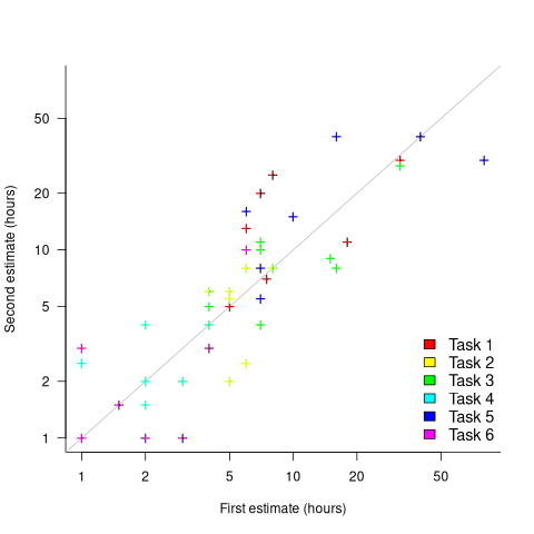
Assuming the estimation uncertainty in this experiment’s data is roughly equal to the estimation uncertainty in other estimation datasets, of tasks taking up to 20 hours, how might it be used to calculate a value for the uncertainty in estimated values?
Two possibilities include:
- Assuming that the uncertainty in both the first and second estimates is equal, a model can be fitted using Deming regression (which treats both variables as having the same uncertainty), and the residual standard error of this model used as the value of
 . This value for a fitted multiplicative model is 0.6 (code+data),
 - using the mean of the relative errors,
 ; its value is 0.55.
How different are the models built using linear regression and errors-in-variables regression, for small task estimates?
A basic linear regression model fitted to the SiP estimation dataset is:  .
.
Updating this model, using SIMEX, to take into uncertainty in the value of  gives, for an uncertainty error of 0.55:
  , and for an uncertainty error of 0.60:
  . The coefficients for the two models are essentially the same (code+data).
The exponent value is the noticeable difference between the linear regression and errors-in-variables regression models. Adding the assumed amount of uncertainty (based on data from one experiment) to the estimated value leads to a model where estimate/actual are very close to having a linear relationship.
Is this errors-in-variables model any closer to reality than the linear regression model? The model shows that the estimate/actual relationship is closer to linear than was previously thought. Until more data becomes available, we won’t know how close this relationship actually is.
The people who made the estimates in the SiP data also performed the work that took the recorded actual time. Assigning a task to a different person could produce both a different estimate and a different actual, but these possible values are unknown. On a larger scale, different companies bidding on the same contract specify different amounts and have different implementations times; data showing these differences.
if statement conditions, some basic measurements
The conditions contained in if-statements control all the decisions a program makes, yet relatively little is known about their characteristics.
A condition contains one or more clauses, for instance, the condition (a && b) contains two clauses that both need to be true, for the condition to be true. An earlier post modelled the number of clauses in Java conditions, and found an exponential decline (around 90% of conditions contained a single clause, for C this is around 85%).
The condition in a nested if-statement contains implicit decisions, because its evaluation depends on the conditions evaluated by its outer if-statements. I have long predicted that, on average, the number of clauses in a condition will decrease as if-statement nesting increases, because some decisions are subsumed by outer conditions. I have not seen any measurements on conditionals vs nesting, and this week this question reached the top of my to-do list.
I used Coccinelle to extract the text contained in each condition, along with the start/end line numbers of the associated if/else compound statement(s). After almost 20 years, Coccinelle is still the most flexible C source analysis tool available that does not require delving into compiler internals. The following is an example of the output (code and data):
file;stmt;if_line;if_col;cmpd_end;cmpd_line_end;expr sqlite-src-3460100/src/fkey.c;if;240;10;240;243;aiCol sqlite-src-3460100/src/fkey.c;if;217;6;217;217;! zKey sqlite-src-3460100/src/fkey.c;if;275;8;275;275;i == nCol sqlite-src-3460100/src/fkey.c;if;1428;6;1428;1433;aChange == 0 || fkParentIsModified ( pTab , pFKey , aChange , bChngRowid ) sqlite-src-3460100/src/fkey.c;if;808;4;808;808;iChildKey == pTab -> iPKey && bChngRowid sqlite-src-3460100/src/fkey.c;if;452;4;452;454;nIncr > 0 && pFKey -> isDeferred == 0 |
The conditional expressions (last column above) were reduced to a basic form involving simple variables and logical operators, along with operator counts. Some example output below (code and data):
simp_expr,land,lor,ternary v1,0,0,0 v1 && v2,1,0,0 v1 || v2,0,1,0 v1 && v2 && v3,2,0,0 v1 || ( v2 && v3 ),1,1,0 ( v1 && v2 ) || ( v3 && v4 ),2,1,0 ( v1 ? dm1 : dm2 ),0,0,1 |
The C source code projects measured were the latest stable versions of Vim (44,205 if-statements), SQLite (27,556 if-statements), and the Linux kernel (version 6.11.1; 1,446,872 if-statements).
A side note: I was surprised to see the ternary operator appearing in some conditions; in effect, an if within an if (see last line of the previous example). The ternary operator usually appears as a component of a large conditional expression (e.g., x + ( v1 ? dm1 : dm2 ) > y), rather than itself containing clauses, e.g., ( v1 ? dm1 : dm2 ) && v2. I have not seen the requirements for this operator discussed in any analysis of MC/DC.
The plot below shows the number of if-statements occurring at a given nesting level, along with regression fits, of the form  , to the Vim and SQLite data; the Linux data was better fit by a power law (code+data):
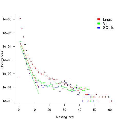
I suspect that most of the deeply nested levels in Vim and SQLite are the results of long else if chains, which, while technically highly nested, could all have been written having the same nesting level, such as the following:
if (strcmp(x, "abc")) ; // code else if (strcmp(x, "xyz")) ; // code else if (strcmp(x, "123")) ; // code |
This if else pattern does not appear to be common in Linux. Perhaps ‘regularizing’ the if else sequences in Vim and SQLite will move the distribution towards a power law (i.e., like Linux).
Average nesting depth will also be affected by the average number of lines per function, with functions containing more statements providing the opportunity for more deeply nested if-statements (rather than calling a function containing nested if-statements).
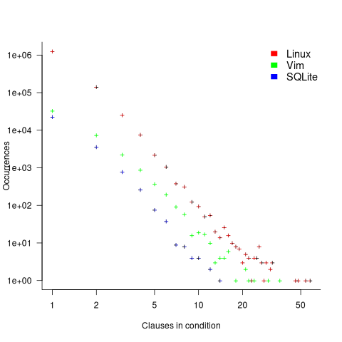
The plot below shows the number of occurrences of conditions containing a given number of clauses. Neither the exponential and power law are good fits, and log-log axis are used because it shows the points are closer to forming a straight line (code+data):
The plot below shows the nesting level and number of clauses in the condition for each of the 1,446,872 if-statements in the Linux kernel. Each value was ‘jittered’ to distribute points about their actual value, creating a more informative visualization (code+data):

As expected, the likelihood of a condition containing multiple clauses does decrease with nesting level. However, with around 85% of conditions containing a single clause, the fitted regression models essential predict one clause for all nesting levels.
MC/DC a step towards safety critical Open source software
Open source projects and safety critical software are at opposite ends of the development process spectrum. From the user perspective, when an Open source project becomes very widely used within its application domain, there is a huge incentive to run it within safety critical domains.
How might software that was not originally developed using a safety critical process be certified for use in a safety critical domain?
A mass of process bureaucracy has sprung up around building software systems whose correct operation is depended on in safety critical situations. There is no evidence that any process bureaucracy produces more reliable software than any other process bureaucracy, and organizations adapt processes to fit within the rules and deliver a system given the available funding.
Some processes specify measurable output requirements, and being able to show that a program developed using an Open source process meets the desired measurable requirements is a step on the path to possible certification. One of the requirements specified in DO-178C (“Software Considerations in Airborne Systems and Equipment Certification”, a non-free publication) for level A: Anomalous behavior produces a catastrophic failure condition, is 100% Modified condition/decision coverage (MC/DC) of the source code. In the automotive world, the same coverage requirement is specified for Automotive Safety Integrity Level D of ISO 26262. As far as I know, the only DO-178C certified Open source program, at this level (which does not imply being safety critical), is SQLite.
The two main hurdles to the adoption of MC/DC by Open source projects are the huge amount of work involved in creating the necessary tests and, until recently, the lack of industrial strength Open source tools for measuring MC/DC (there are many commercial tools).
While compiler support for statement coverage has long been available in both GCC and clang, support for MC/DC only became available in an official release of clang this year (the initial functionality was pushed in 2021). The official releases of GCC do not yet support MC/DC, but a patch has been available since 2022 (talk by author).
Making available an industrial strength Open source compiler that supports MC/DC testing removes one barrier on the path to DO-178C certification of Open source programs. The certification process itself requires that support tools meet certain minimum requirements, which are specified in DO-330. A tool used as part of the verification process of a program at Level A needed not itself have 100% MC/DC, or even 100% statement coverage. The LLVM project tracks statement coverage, which is not even close to 100%.
Are there any coding constructs that get in the way of achieving 100% MC/DC?
It’s possible to write a condition that cannot be tested in a way that meets the MC/DC requirement: Each condition in a decision is shown to independently affect the outcome of the decision. For instance, in the following condition:
if ((A && B) || (!A && C)) |
the value of the variable A affects the outcome of both operands of ||, and the complete expression cannot be rewritten, using just A, B, C, to change this situation. The complete boolean expression is said to be strongly coupled. An expression involving the same variable in multiple relational or equality tests (e.g., (x > 0) && (x < 10)) is said to be weakly coupled.
An analysis of the Ada source code (appendix C) contained in five aircraft flight recorders finds examples of strongly and weakly coupled conditions. This suggests that occurrences of these construct in source code does not prevent a program becoming DO-178C certified.
Linux must be the prime candidate for an Open source program being considered for some kind of safety critical certification. A kernel patch to support MC/DC profiling is in the works (with a kernel MC/DC of around 2.33%, lots of new tests are going to have to be written). Lots of other significant certification requirements also need to be met.
In C, around 90% of if-statements contain a single conditional test (statement 1739), while in Java around 90% of if-statements contain a single conditional test, with around 0.1% containing five or more.
A kind of coverage that is not so often discussed is object code structural coverage, i.e., coverage based on the conditions contained in generated machine code, such as from a compiler. Object code coverage is designed to handle the possibility of compilers generating code containing conditions that are not present in the original source.
Some compilers generate the same machine code for both top level if-statements in the following code:
int g; void square(int a, int b, int c) { if (a && b && c) g++; if (a) if (b) if (c) g++; } |
Modeling program LOC growth with recurrence equations
Models predicting the growth, in lines of code, of a program are based on the assumption that future growth follows the same pattern of behavior as past growth. One such model is the recurrence relation:
 , where:
  is LOC at time
  ,
,  is the LOC carried over from release
  , and
, and  is the LOC added after release
  .
.
The solution to this recurrence relation is:  , where:
  is the LOC at time
  .
.
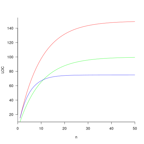
The plot below shows the growth predicted by this model, for various values of  and
and  (code+data):
How close is the fit between this model and actual project growth? The plot below shows the growth in LOC for FreeBSD between 1993 and 2006, data from Herraiz; the red line shows the above equation fitted using non-linear regression, with the blue line showing a fitted linear regression model of the form  (code+data):
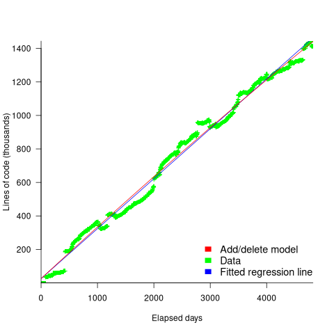
Plugging the fitted coefficients into the recurrence equation when  gives a prediction for the final maximum LOC in FreeBSD of:

The FreeBSD growth is unusual in not having a slow start to its growth, or rather no data is available prior to 1993.
Long-lived, successful projects usually attract new developers, and over time some developers leave. The size of a project, and the predispositions of those involved, can limit the number of active core developers. The above model can be applied to the growth in the number of active developers, i.e.,
 , where:
  is active developers at time
  ,
,  is the developers ceasing to be active
  , and
, and  is the number of new active developers at
  . The solution is:

Adding the developer growth equation in to the LOC model, we get:
 , where
  is now multiplied by the number of developers at time
  , i.e.,
  . The solution to these recurrence equations is somewhat involved (note: if you are using an LLM to check the answers, ChatGPT makes multiple mistakes, but the Grok response contains just one algebra mistake); when
  the equation is:

Checking this more complicated model against another project, the plot below shows the growth of the GNU C library between 1990 and 2011, data from Gonzalez-Barahona, Robles, Herraiz and Ortega; the red line is the fitted equation  (code+data):
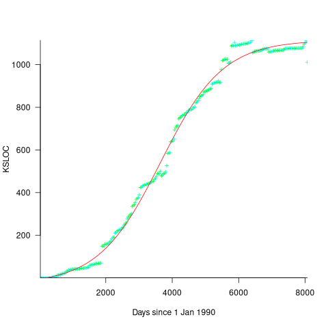
Unsurprisingly, I was not able to fit the more complicated growth model, using non-linear least squares, to the glibc LOC data. The problem was not being able to mimic the slow initial growth rate. I suspect that the developer growth model might be just wrong. Development work on a project does not last forever, and the number of developers will start decreasing at some point. For large projects, the Rayleigh distribution has been found to approximate staffing levels.
Data on project developer numbers over time is rare. The Linux kernel data shows an exponential developer growth rate, but I suspect that this is mostly caused by many one-time only developer contributing towards a new device driver (which are responsible for much of the Kernel growth).
Discussing new language features is more fun than measuring feature usage in code
How often are the features supported by a programming language used by developers in the code that they write?
This fundamental question is rarely asked, let alone answered (my contribution).
Existing code is what developers spend their time reading, compilers translating to machine code, and LLMs use as training data.
Frequently used language features are of interest to writers of code optimizers, who want to know where to focus their limited resources (at least I did when I was involved in the optimization business; I was always surprised by others working in the field having almost no interest in measuring user’s code), and educators ought to be interested in teaching what students are mostly likely to be using (rather than teaching the features that are fun to talk about).
The unused, or rarely used language features are also of interest. Is the feature rarely used because developers have no use for the feature, or does its semantics prevent it being practically applied, or some other reason?
Language designers write books, papers, and blog posts discussing their envisaged developer usage of each feature, and how their mental model of the language ties everything together to create a unifying whole; measurements of actual source code very rarely get discussed. Two very interesting reads in this genre are Stroustrup’s The Design and Evolution of C++ and Thriving in a Crowded and Changing World: C++ 2006–2020.
Languages with an active user base are often updated to support new features. The ISO C++ committee is aims to release a new standard every three years, Java is now on a six-month release cycle, and Python has an annual release cycle. The primary incentives driving the work needed to create these updates appears to be:
- sales & marketing: saturation exposure to adverts proclaiming modernity has warped developer perception of programming languages, driving young developers to want to be associated with those perceived as modern. Companies need to hire inexperienced developers (who are likely still running on the modernity treadmill), and appearing out of date can discourage developers from applying for a job,
- designer hedonism and fuel for the trainer/consultant gravy train: people create new programming languages because it’s something they enjoy doing; some even leave their jobs to work on their language full-time. New language features provides material to talk about and income opportunities for trainers/consultants.
Note: I’m not saying that adding new features to a language is bad, but that at the moment worthwhile practical use to developers is a marketing claim rather than an evidence-based calculation.
Those proposing new language features can rightly point out that measuring language usage is a complicated process, and that it takes time for new features to diffuse into developers’ repertoire. Also, studying source code measurement data is not something that appeals to many people.
Also, the primary intended audience for some language features is library implementors, e.g., templates.
There have been some studies of language feature usage. Lambda expressions are a popular research subject, having been added as a new feature to many languages, e.g., C++, Java, and Python. A few papers have studied language usage in specific contexts, e.g., C++ new feature usage in KDE.
The number of language features invariably grow and grow. Sometimes notice is given that a feature will be removed from a future reversion of the language. Notice of feature deprecation invariably leads to developer pushback by the subset of the community that relies on that feature (measuring usage would help prevent embarrassing walk backs).
If the majority of newly written code does end up being created by developers prompting LLMs, then new language features are unlikely ever to be used. Without sufficient training data, which comes from developers writing code using the new features, LLMs are unlikely to respond with code containing new features.
I am not expecting the current incentive structure to change.
Number of statement sequences possible using N if-statements
I recently read a post by Terence Tao describing how he experimented with using ChatGPT to solve a challenging mathematical problem. A few of my posts contain mathematical problems I could not solve; I assumed that solving them was beyond my maths pay grade. Perhaps ChatGPT could help me solve some of them.
To my surprise, a solution was found to the first problem I tried.
I simplified the original problem (involving Motzkin numbers, details below) down to something that was easier for me to explain to ChatGPT. Based on ChatGPT’s response, it appeared lost, so I asked what it knew about Motzkin numbers. I then reframed the question around the concepts in its response, and got a response that, while reasonable, was not a solution. My question was not precise enough, and a couple of question/answer iterations later, ChatGPT broke the problem down into a series of steps that I saw could solve the problem. While the equation it used in its answer was just wrong, I knew what the correct equation was. So while ChatGPT frequently went off in the wrong direction and got its maths wrong, it helped me refine my statement of the problem and ChatGPT eventually gave steps to a solution which were blindingly obvious to me when I read them.
The question I wanted to answer was: How many distinct statement sequences can be created using 
if-statements and  simple-statements (for a total of
  statements)?
A simple-statement might be an assignment or function call, but not any kind of compound statement, such as a loop. Three sequences are possible using one if-statement and two simple-statements. The if-statement occupies two lines, i.e., the condition and termination curly-bracket, }, as follows:
s1; if (c1) { if (c1) { if (c1) { s1; s1; s2; s2; } } } s2; |
In a previous post I showed how a variant of this question, involving any number of if-statements, can be mapped to a combinatorial interpretation of Motzkin numbers and treating matching up/down diagonals along a path as an if-statement.
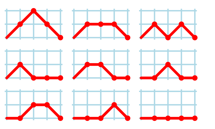
ChatGPT performed poorly when I phrased the problem in combinatorial terms (or perhaps my phrasing was poor), so I switched to using a lattice path approach. I asked: “How many lattice paths of length S containing exactly N occurrences of the step (1, 1) and N occurrences of the step (1, -1) are possible?”, and after reading the response I replied “Your analysis does not take into account the fact that the path cannot go below the x-axis. Rework your analysis to take this restriction into account.”
The following is my edited version of ChatGPT’s ‘solution’ response:
“Problem Restated:
We need to count the number of valid Dyck paths of length  , where the path consists of:
Exactly  upward steps (1,1).
Exactly  downward steps (1,−1).
The remaining steps (which must be  horizontal steps (1,0)).
These paths must never dip below the x-axis, and they must return to the x-axis at the end.
…
Step 2: Catalan Numbers for Balanced Paths
If we ignore the horizontal steps for the moment, the number of ways to place  upward steps and
  downward steps such that the path does not go below the x-axis is given by the Catalan number
  :
:

This Catalan number counts the number of valid ways to arrange the  upward steps and
  downward steps such that the path remains above or on the x-axis.
Step 3: Placing Horizontal Steps
Once the valid upward and downward steps have been arranged in a Catalan structure, we can freely place the  horizontal steps (1,0) in the remaining positions of the path. Since there are
  steps (upward and downward) and
  horizontal steps, there are
  gaps (before, after, or between the upward/downward steps) where the horizontal steps can be placed.
The number of ways to place  horizontal steps in these
  positions is given by a binomial coefficient:”
For some reason, ChatGPT gives the wrong binomial coefficient. Calculating the number of ways of distributing  items into
  bins is a well known problem; when a bin can contain zero items, the solution is:
  .
.
Combining the equations from the two steps gives the number of distinct statement sequences that can be created using 
if-statements and  simple-statements as:

The above answer is technically correct, however, it fails to take into account that in practice an if-statement body will always contain either another if-statement or a simple statement, i.e., the innermost if-statement of any nested sequence cannot be empty (the equation used for distributing items into bins assumes a bin can be empty).
Rather than distributing  statements into
  gaps, we first need to insert one simple statement into each of the innermost if-statements. The number of ways of distributing the remaining statements are then counted as previously. How many innermost if-statements can be created using
  if-statements? I found the answer to this question in a StackExchange question, using traditional search.
The question can be phrased in terms of peaks in Dyck paths, and the answer is contained in the Narayana numbers (which I had never heard of before). The following example, from Wikipedia, shows the number of paths containing a given number of peaks, that can be produced by four if-statements:
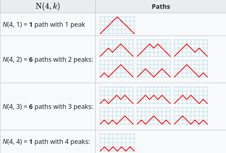
The sum of all these paths is the Catalan number for the given number of if-statements, e.g., using  to denote the Narayana number:
  .
.
Adding at least one simple statement to each innermost if-statement changes the equation for the number of statement sequences from  , to:
, to:

The following table shows the number of distinct statement sequences for five-to-twenty statements containing one-to-five if-statements:
                   N if-statements
           1       2       3       4       5
   5       6       1
   6      10       6
   7      15      20       1
   8      21      50       7
   9      28     105      29       1
  10      36     196      91       9
  11      45     336     238      45       1
  12      55     540     549     166      11
S 13      66     825   1,155     504      66
  14      78   1,210   2,262   1,332     286
  15      91   1,716   4,179   3,168   1,002
  16     105   2,366   7,351   6,930   3,014
  17     120   3,185  12,397  14,157   8,074
  18     136   4,200  20,153  27,313  19,734
  19     153   5,440  31,720  50,193  44,759
20 171 6,936 48,517 88,458 95,381 |
The following is an R implementation of the calculation:
Narayana=function(n, k) choose(n, k)*choose(n, k-1)/n

Catalan=function(n) choose(2*n, n)/(n+1)


if_stmt_possible=function(S, N)
{
return(Catalan(N)*choose(S, 2*N)) # allow empty innermost if-statement
}


if_stmt_cnt=function(S, N)
{
if (S <= 2*N)
   return(0)
total=0
for (k in 1:N)
   {
   P=Narayana(N, k)
   if (S-P*k >= 2*N)
      total=total+P*choose(S-P*k, 2*N)
   }

return(total)
}

isc=matrix(nrow=25, ncol=5)

for (S in 5:20)
   for (N in 1:5)
      isc[S, N]=if_stmt_cnt(S, N)

print(isc) |
Measuring non-determinism in the Linux kernel
Developers often assume that it’s possible to predict the execution path a program will take, for a given set of input values, i.e., program behavior is deterministic. The execution path may be very complicated, and may depend on the contents of certain files (e.g., SQL engines), but it’s deterministic.
There is one kind of program where determinism is not an option; operating systems are non-deterministic when running in a mode where interrupts can occur.
How much non-determinism can occur in, say, Linux? For instance, when a program calls a system function (e.g., open, read, write, close), how often does the execution sequence follow the function call tree that appears in the source code, and how many different call sequences actually occur during program execution (because of diversions caused by an interrupt; ignoring control flow within functions)?
A study by Imanol Allende ran the same program 500K+ times, and traced every function call that occurred within the Linux kernel (thanks to Imanol for sending me the data and answering my questions). The program used appears below; the system calls traced were open (two distinct calls), read, write, and close (two distinct calls); a total of six system calls.
// #includes omitted int main(int argc, char **argv) { unsigned char result; int fd1, fd2, ret; char res_str[10]={0}; fd1 = open("/dev/urandom", O_RDONLY); fd2 = open("/dev/null", O_WRONLY); ret = read(fd1 , &result, 1); sprintf(res_str ,"%d", result); ret = write(fd2, res_str, strlen(res_str)); close(fd1); close(fd2); return ret; } |
Analysing each of these six distinct calls, in around 98% of program runs, each call follows the same sequence of function calls within the kernel (the common case for write involves a chain of around 10 function calls). During the other 2’ish% of calls, the common sequence was interrupted for some reason, and the logged call trace includes additional called functions, e.g., calls involving the Read, Copy, Update synchronization mechanism. The plot below shows the growth in the number of unique traces against the number of program runs (436,827 of them) for the close(fd2) call; a fitted regression line is in red, with the first 1,000 runs not included in the fit (code+data):

The fitted regression model is  , suggesting that the growth in unique traces is slowing (this equation peaks at around
  ), while the model fitted to some of the system calls implies ever continuing growth.
Allende investigated more sophisticated techniques for estimating the total number of unique traces, including: extreme value theory and species estimation techniques from ecology.
While around 98% of traces are the common case, over half of the unique traces occurred once in 436,827 runs. The plot below shows the number of occurrences of each unique trace, for the close(fd2) call, with an attempted fit of a bi-exponential model (in red; code+data):
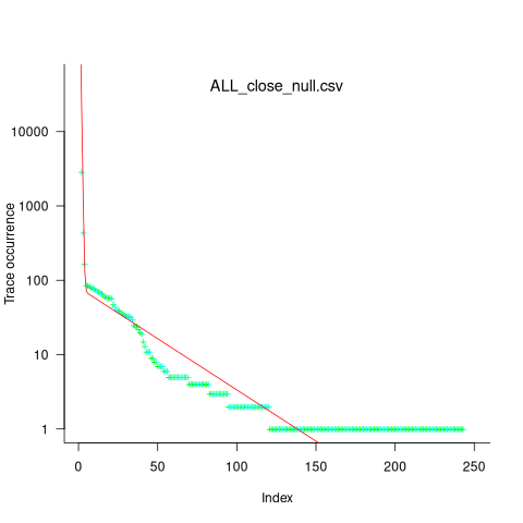
The analysis above looked at one system call, the program contains six system calls. If, for each system call, the probability of the most common trace is 98%, then the probability of all six calls following their respective common case is 89%. As the number of distinct system calls made by a program goes up, the global common case becomes less common, and the number of distinct program traces increases multiplicatively.
Survival of CVEs in the Linux kernel
Software contained in safety related applications has to have a very low probability of failure.
How is a failure rate for software calculated?
The people who calculate these probabilities, or at least claim that some program has a suitably low probability, don’t publish the details or make their data publicly available.
People have been talking about using Linux in safety critical applications for over a decade (multiple safety levels are available to choose from). Estimating a reliability for the Linux kernel is a huge undertaking. This post is taking a first step via a broad brush analysis of a reliability associated dataset.
Public fault report logs are a very messy data source that needs a lot of cleaning; they don’t just contain problems caused by coding mistakes, around 50% are requests for enhancement (and then there is the issue of multiple reports having the same root cause).
CVE number are a curated collection of a particular kind of fault, i.e., information-security vulnerabilities. Data on 2,860 kernel CVEs is available. The data includes the first released version of the kernel containing the problem, and the version of the fixed release. The plot below shows the survival curve for kernel CVEs, with confidence intervals in blue/green (code+data):

The survival curve appears to have two parts: the steeper decline during the first 1,000 days, followed by a slower, constant decline out to 16+ years.
Some good news is that many of these CVEs are likely to be in components that would not be installed in a safety critical application.
Recent Comments