Archive
Changing development culture and practices: LLM edition
The popular perception of creating software systems is that it mainly involves writing code. In the 1950s, management treated writing code as a clerical task that just mapped the detailed requirements specified by someone with knowledge of the problem to something a computer could execute. Job titles reflected this division of labour, e.g., coder/programmer, systems analyst (the Wikipedia entry lists implementation as part of the job, this eventually became true in theory and for many was probably true in practice since the early days).
Using Large Language Models to write code based on the requirements contained in a prompt appears to take software development back to the process mandated by the managers of early software projects.
A major economic incentive for the creation of software systems is enabling more efficient work processes, with the collateral damage of decimated employment in some work functions. This happened to clerical workers and non-software engineering workers. Now it’s happening to software developers.
Hardware designers did not cease to exist once Computer-aided design became available. Technical drawing skills (larger schools once had a room full of drawing boards for teaching young teenagers) has ceased to be a job requirement (image from Wikipedia).

Software developer will remain as a job category, perhaps with reduced numbers or with reduced average pay. But the use of LLMs will change the culture and practices of software development.
The shift from using assembly language to high level languages suggests a few ideas about the kinds of changes. Using assembly language requires being reasonably familiar with the cpu architecture, e.g., register names/widths/instruction-restrictions and instruction timings. General developer chat about cpu architectures was still a thing in the 1980s, less so in the 1990s, and very rarely today (people do blog about it). Several decades from now, what will no longer be a general topic of developer conversation? Data types, perhaps; like registers, bit pattern representation is a low level detail. Since most developers don’t know much about the languages they use, it may be difficult to measure the impact of LLM usage on language knowledge.
High-level languages increase developer productivity by reducing the number of details that need to be thought about, at the cost of less efficient code. But for many applications, machine time is cheaper than human time.
LLMs increase developer productivity by reducing the need to lookup details (e.g., spelling of method names and their parameters). As confidence grows in the accuracy of LLM suggested code, developers will start accepting, whatever. What counts is whether the code works, not whether the average developer would have written something faster/smaller/idiomatic.
The early languages have a straightforward mapping from statements/declarations to machine code. Over time, languages were created that allowed developers to think less and less about implementation details, at the cost of supporting constructs that could introduce lots of hidden overhead. I expect that customer demand will incentivize LLM functionality that reduces what developers need to think about.
A real danger of LLM usage is that it will, eventually, result in programs a lot more bloated than humans have managed to achieve. There are physical constraints restricting what hardware designers can do, and these constraints show up in patterns of behavior, e.g., Rent’s rule relating the number of external connections in a logic block to the number of logic gates in the block. There are common usage patterns in existing code, but no theory suggesting they are desirable, or not, in any sense. I await having enough LLM generated production code to make statistically significant measurements.
I suspect that these days most developers are writing glue code, or short programs, and in the near term I expect that most LLM code will fill this need. Unfortunately, there is very little research/measurement on glue code/short program, so there are no known developer usage patterns to compare LLMs against.
My 2024 in software engineering
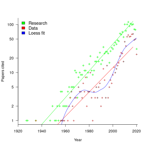
Readers are unlikely to have noticed something that has not been happening during the last few years. The plot below shows, by year of publication, the number of papers cited (green) and datasets used (red) in my 2020 book Evidence-Based Software Engineering. The fitted red regression lines suggest that the 20s were going to be a period of abundant software engineering data; this has not (yet?) happened (the blue line is a local regression fit, i.e., loess). In 2020 COVID struck, and towards the end of 2022 Large Language Models appeared and sucked up all the attention in the software research ecosystem, and there is lots of funding; data gathering now looks worse than boring (code+data):
LLMs are showing great potential as research tools, but researchers are still playing with them in the sandpit.
How many AI startups are there in London? I thought maybe one/two hundred. A recruiter specializing in AI staffing told me that he would estimate around four hundred; this was around the middle of the year.
What did I learn/discover about software engineering this year?
Regular readers may have noticed a more than usual number of posts discussing papers/reports from the 1960s, 1970s and early 1980s. There is a night and day difference between software engineering papers from this start-up period and post mid-1980s papers. The start-up period papers address industry problems using sophisticated mathematical techniques, while post mid-1980s papers pay lip service to industrial interests, decorating papers with marketing speak, such as maintainability, readability, etc. Mathematical orgasms via the study of algorithms could be said to be the focus of post mid-1980s researchers. So-called software engineering departments ought to be renamed as Algorithms department.
Greg Wilson thinks that the shift happened in the 1980s because this was the decade during which the first generation of ‘trained in software’ people (i.e., emphasis on mathematics and abstract ideas) became influential academics. Prior generations had received a practical training in physics/engineering, and been taught the skills and problem-solving skills that those disciplines had refined over centuries.
My research is a continuation of the search for answers to the same industrial problems addressed by the start-up researchers.
In the second half of the year I discovered the mathematical abilities of LLMs, and started using them to work through the equations for various models I had in mind. Sometimes the final model turned out to be trivial, but at least going through the process cleared away the complications in my mind. According to reports, OpenAI’s next, as yet unreleased, model has super-power maths abilities. It will still need a human to specify the equations to solve, so I am not expecting to have nothing to blog about.
Analysis/data in the following blog posts, from the last 12-months, belongs in my book Evidence-Based Software Engineering, in some form or other:
Small business programs: A dataset in the research void
Putnam’s software equation debunked (the book is non-committal).
if statement conditions, some basic measurements
Number of statement sequences possible using N if-statements; perhaps.
A new NASA software dataset from the 1970s
A surprising retrospective task estimation dataset
Average lines added/deleted by commits across languages
Census of general purpose computers installed in the 1960s
Some information on story point estimates for 16 projects
Agile and Waterfall as community norms
Median system cpu clock frequency over last 15 years
The evidence-based software engineering Discord channel continues to tick over (invitation), with sporadic interesting exchanges.
Small business programs: A dataset in the research void
My experience is that most of the programs created within organizations are very short, i.e., around 50–100 lines. Sometimes entire businesses are run using many short programs strung together in various ways. These short programs invariably make extensive use of the functionality provided by a much larger package that handles all the complicated stuff.
In the software development world, these short programs are likely to be shell scripts, but in the much larger ecosystem that is the business world these programs will be written in what used to be called a fourth generation language (4GL). These 4GLs are essentially domain specific languages for specific business tasks, such as report generation, or database query products, and for some time now spreadsheets.
The business software ecosystem is usually only studied by researchers in business schools, but short programs, business or otherwise, are rarely studied by any researchers. The source of such short programs is rarely publicly available; even if the information is not commercially confidential, the program likely addresses one group’s niche problem which is of no interest to anybody else, i.e., there is no rationale to publishing it. If source were available, there might not be enough of it to do any significant analysis.
I recently came across Clive Wrigley’s 1988 PhD thesis, which attempts to build a software estimation model. It contains summary data of 26 transaction processing systems written in the FOCUS language (an automated code generator).
For many organizations, there is a fundamental difference between business related problems and scientific/engineering problems, in that business problems tend to involve simple operations on lots of distinct data items (e.g., payroll calculation for each company employee), while scientific/engineering often involves a complicated formula operating on one set of data. There are exceptions.
4GLs enable technically proficient business users to create and maintain good enough applications without needing software engineering skills (yes, many do create spaghetti code), because they are not writing thousands of lines of code. The applications often contain many semi-self-contained subcomponents, which can be shared or swapped in/out. The small size makes it easier to change quickly, and there is direct access to the business users, it’s an agile process decades before this process took off in the world of non-4GL languages.
A major claim made by fans of 4GL is that it is much cheaper to create applications equivalent to those created using a 3GL, e.g., Cobol/C/C++/Java/Python/etc. I would agree that this true for small applications that fit the use-case addressed by a particular 4GL, but I think the domain specific nature of a 4GL will limit what can be done and likely need to be done in larger applications.
How do 4GL applications written in FOCUS compare against application written in Cobol? A 1987 paper by Chris Kemerer provides some manpower/LOC data for Cobol applications. I have no information on the amount of functionality in any of the applications. The plot below shows developer hours consumed creating 26 systems containing a given number of lines of code for FOCUS (green) and 15 COBOL (blue) programs, with fitted regression models in red (code+data):
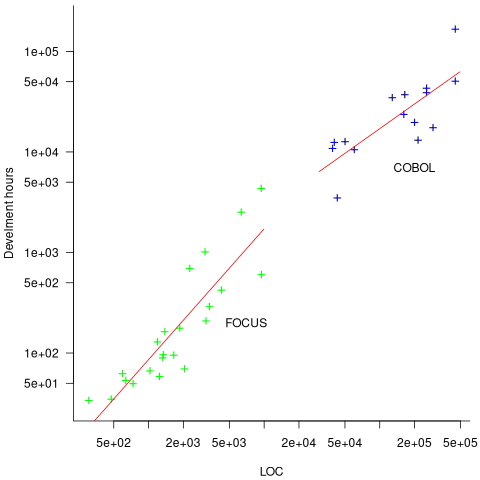
The two samples of applications differ by two orders of magnitude in LOC and developer hours, however, there is no information on the functionality provided by the applications.
Good enough reliability models: still an unknown
Estimating the likelihood that a software system will operate as intended, for some period of time, is one of the big problems within the field of software reliability research. When software does not operate as intended, a fault, or bug, or hallucination is said to have occurred.
Three events need to occur for a user of a software system to experience a fault:
- a developer writes code that does not always behave as intended, i.e., a coding mistake,
- the user of the software feeds it input that causes the coding mistake to produce unintended behavior,
- the unintended behavior percolates through the system to produce a visible fault (sometimes an unintended behavior does not percolate very far, and does not produce any change of visible behavior).
Modelling each kind of event and their interaction is a huge undertaking. Researchers in one of the major subfields of software reliability take a global approach, e.g., they model time to next fault experience, using data on the number of faults experienced per given amount of cpu/elapsed time (often obtained during testing). Modelling the fault data obtained during testing results in a model of the likelihood of the next fault experienced using that particular test process. This is useful for doing a return-on-investment calculation to decide whether to do more testing. If the distribution of inputs used during testing is similar to the distribution of customer inputs, then the model can be of use in estimating the rate of customer fault experiences.
Is it possible to use a model whose design was driven by data from testing one or more software systems to estimate the rate of fault experiences likely when testing other software systems?
The number of coding mistakes will differ between systems (because they have different sizes, and/or different developer abilities), and the testers’ ability will be different, and the extent to which mistaken behavior percolates through code will differ. However, it is possible for there to be a general model for rate of fault experiences that contains various parameters that need to be fitted for each situation.
Since that start of the 1970s, researchers have been searching for this general model (the first software reliability model is thought to be: “Program errors as a birth-and-death process” by G. R. Hudson, Report SP-3011, System Development Corp., 1967 Dec 4; please send me a copy, if you have one).
The image below shows the 18 models discussed in the 1987 book “Software Reliability: Measurement, Prediction, Application” by Musa, Iannino, and Okumoto (later editions have seriously watered down the technical contents, and lack most of the tables/plots). It’s to be expected that during the early years of a new field, many different models will be proposed and discussed.
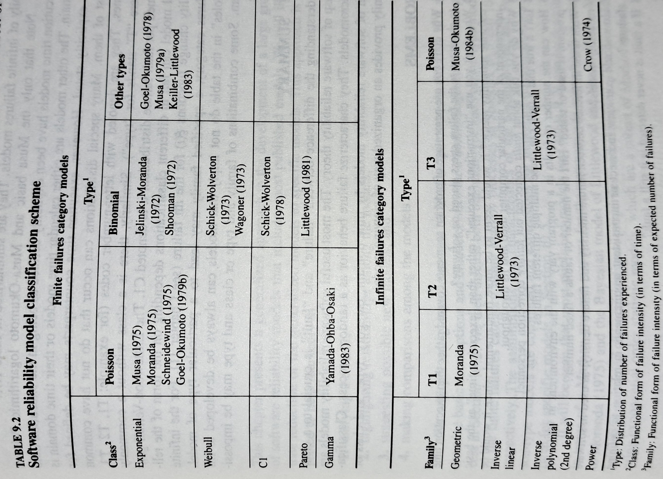
Did researchers discover a good-enough general model for rate of fault experiences?
It’s hard to say. There is not enough reliability data to be confident that any of the umpteen proposed models is consistently better at predicting than any other. I believe that the evidence-based state of the art has not yet progressed beyond the 1982 report Software Reliability: Repetitive Run Experimentation and Modeling by Nagel and Skrivan.
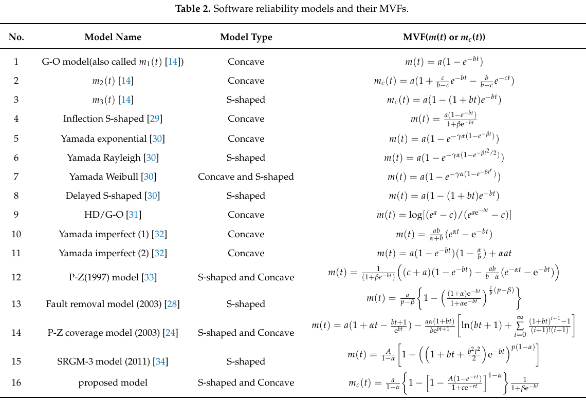
Fitting slightly modified versions of existing models to a small number of tiny datasets has become standard practice in this corner of software engineering research (the same pattern of behavior has occurred in software effort estimation). The image below shows 16 models from a 2021 paper.
Nearly all the reliability data used to create these models is from systems built in the 1960s and 1970s. During these decades, software systems were paid for organizations that appreciated the benefits of collecting data to build models, and funding the necessary research. My experience is that few academics make an effort to talk to people in industry, which means they are unlikely to acquire new datasets. But then researchers are judged by papers published, and the ecosystem they work within is willing to publish papers extolling the virtues of another variant of an existing model.
The various software fault datasets used to create reliability models tends to be scattered in sometimes hard to find papers (yes, it is small enough to be printed in papers). I have finally gotten around to organizing all the public data that I have in one place, a Reliability data repo on GitHub.
If you have a public fault dataset that does not appear in this repo, please send me a copy.
Christmas books for 2024
My rate of book reading has picked up significantly this year. The following are the really interesting books I read, as is usually the case, most were not published in this year.
I have enjoyed Grayson Perry’s TV programs on the art world, so I bought his book “Playing to the Gallery: Helping Contemporary Art in its Struggle to Be Understood“. It’s a fun, mischievous look at the art world by somebody working as a traditional artist, in the sense of creating work that they believe means/says something, rather than works that are only considered art because they are displayed in an art gallery.
“The Computer from Pascal to von Neumann” by H. H. Goldstine. This history of computing from the mid-1600s (the time of Blaise Pascal) to the mid-1900s (von Neumann died in 1957) told by a mathematician who was first involved in calculating artillery firing tables during World War II, and then worked with early computers and von Neumann. This book is full of insights that only a technical person could provide and is a joy to read.
I saw a poster advertising a guided tour of the trees in my local park, organized by Trees for Cities. It was a very interesting lunchtime; I had not appreciated how many different trees were growing there, including three different kinds of Oak tree. Trees for Cities run events all over the UK, and abroad. Of course, I had to buy some books to improve my tree recognition skills. I found “Collins tree guide” by O. Johnson and D. More to be the most useful and full of information. Various organizations have created maps of trees in cities around the world. The London Tree Map shows the location and species information for over 880,000 of trees growing on streets (not parks), New York also has a map. For a general analysis of patterns of tree growth, see “How to Read a Tree” by T. Gooley.
“Medieval Horizons: Why the Middle Ages Matter” by I. Mortimer. This book takes the reader through the social, cultural and economic changes that happened in England during the Middle Ages, which the author specifies as the period 1000 to 1600. I knew that many people were surfs, but did not know that slaves accounted for around 10% of the population, dropping to zero percent during this period. Changes, at least for the well-off, included moving from living in longhouses to living in what we would call a house, art works moved from two-dimensional representations to life-like images (e.g., renaissance quality), printing enables an explosion of books, non-poor people travelled more, ate better, and individualism started to take-off.
Statistical Consequences of Fat Tails: Real World Preasymptotics, Epistemology, and Applications by N. N. Taleb is a mathematically dense book (while the pdf is in color, I was disappointed that the printed version is black/white; this is the one I read while travelling). This book tells you a lot more than you need to know about the consequences of fat tail distributions. Why might you be interested in the problems of fat tails? Taleb starts by showing how little noise it takes for the comforting assumptions implied by the Normal/Gaussian distribution to fly out the window. The primary comforting assumptions are that the mean and variance of a small sample are representative of the larger population. A world of fat tail distributions is one where the unexpected is to be expected, where a single event can wipe out an organization or industry (banks are said to have lost more in the 2008 financial crisis than they had made in the previous many decades). This book is hard going, and I kept at it to get a feel for the answers to some of the objections to the bad news conveyed. There are a couple of places where I should have been more circumspect in my Evidence-based software engineering book.
I have previously reviewed General Relativity: The Theoretical Minimum by Susskind and Cabannes.
“Embracing Defeat: Japan in the Wake of World War II” by John W. Dower describes in harrowing detail the dire circumstances of the population of Japan immediately after World War II and what they had to endure to survive.
For more detailed book reviews, see: Mr. and Mrs. Psmith’s Bookshelf with some excellent and insightful long book reviews, and the annual Astral Codex Ten book review contest usually has a few excellent reviews/books.
For those of you who think that civilization is about to collapse, or at least like talking about the possibility, a reading list. At the practical level, I think sword fighting and archery skills are more likely to be useful in the longer term.
21 Algol 60 compilers in 1962
The specification of ALGOL 60 was published in May 1960. Unlike today, where the creators of a new language release the source of a corresponding compiler, people were expected to write their own compiler. The June 1962 paper: The Replies to the AB14 Questionnaire lists implementation details on 21’ish compilers (it’s not clear whether some are dialects or languages very similar to Algol 60; 1963: list of 32 Algol compilers/versions).
Compiler writing was a hot leading edge research topic in the 1960s; at the start of this decade all the techniques we take for granted today had not yet been invented (Knuth invented LR parsing in 1965, and algorithms for optimal code generation started appearing in 1970). The 1960s was the period of the Cambrian explosion for programming languages.
Implementors not only had to deal with all the unknowns of writing a compiler, they also had to do the work using systems whose memory was measured in tens of kilobytes, computer interaction probably via punched card or punched tape, or if lucky, the luxury of teletype input/output. It’s no surprise that fourteen of the implementations considered themselves to be a “true subset” (which I take to mean that everything implemented was as per the specification). Compilers for earlier languages probably had the benefit of the language not supporting anything that was hard to implement.
Compiler implementation know-how received a major boost in 1964 with the publication of the book ALGOL 60 Implementation.
The plot below shows the number of compilers having a given reported implementation time (code+data):
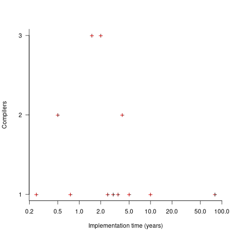
The median implementation effort is 2 man-years. Is this the result of a few good people working off the clock to create software, or management supporting the creation of a product that customers are not clamouring for?
The 0.25 man-year implementation looks like a port of an existing compiler to a different version of the same hardware. The 10 man-year implementation time was for what looks like a full implementation, plus extensions. The 80 man-year implementation time was reported by SDC (a large defence contractor) for a range of JOVIAL compilers (derived from Algol 58) targetting five different hardware platforms.
Were the implementors of Algol compilers different from the implementors of other languages? It’s not possible to say, although the language was created by a distinct group of people. The definition of Algol 60 was created by a committee composed of computing academics and like-minded people, while Fortran was dominated by the major computer company of the day, IBM (1963: list of 51 Fortran compilers; 1964: at least 43 Fortran compilers/versions), and COBOL was designed to be used by those strange business people (1963: list of 37 COBOL implementations/versions).
The Norden-Rayleigh model: some history
Since it was created in the 1960s, the Norden-Rayleigh model of large project manpower has consistently outperformed, or close runner-up, other models in benchmarks (a large project is one requiring two or more man-years of effort). The accuracy of the Norden-Rayleigh model comes with a big limitation: a crucial input value to the calculation is the time at which project manpower peaks (which tends to be halfway through a project). The model just does not work for times before the point of maximum manpower.
Who is the customer for a model that predicts total project manpower from around the halfway point? Managers of acquisition contracts looking to evaluate contractor performance.
Not only does the Norden-Rayleigh model make predictions that have a good enough match with reality, there is some (slightly hand wavy) theory behind it. This post delves into Peter Norden’s derivation of the model, and some of the subsequent modifications. Norden work is the result of studies carried out at IBM Development Laboratories between 1956 and 1964, looking for improved methods of estimating and managing hardware development projects; his PhD thesis was published in 1964.
The 1950s/60s was a period of rapid growth, with many major military and civilian systems being built. Lots of models and techniques were created to help plan and organise these projects, two that have survived the test of time are the critical path method and PERT. As project experience and data accumulated, techniques evolved.
Norden’s 1958 paper “Curve Fitting for a Model of Applied Research and Development Scheduling” describes how a project consists of overlapping phases (e.g., feasibility study, deign, implementation, etc), each with their own manpower rates. The equation Norden fitted to cumulative manpower was:  , where
  is project elapsed time,
  is total project manpower, and
  ,
,  , and
, and  are fitted constants. This is the logistic equation with added tunable parameters.
By the early 1960s, Norden had brought together various ideas to create the model he is known for today. For an overview, see his paper (starting on page 217): Project Life Cycle Modelling: Background and Application of the Life Cycle Curves.
The 1961 paper: “The decisions of engineering design” by David Marples was influential in getting people to think about project implementation as a tree-like collection of problems to be solved, with decisions made at the nodes.
The 1958 paper: The exponential distribution and its role in life testing by Benjamin Epstein provides the mathematical ideas used by Norden. The 1950s was the decade when the exponential distribution became established as the default distribution for hardware failure rates (the 1952 paper: An Analysis of Some Failure Data by D.J. Davis supplied the data).
Norden draws a parallel between a ‘shock’ occurring during the operation of a device that causes a failure to occur and a discovery of a new problem to be solved during the implementation of a task. Epstein’s exponential distribution analysis, along with time dependence of failure/new-problem, leads to the Weibull distribution. Available project manpower data consistently fitted a special case of the Weibull distribution, i.e., the Rayleigh distribution (see: Project Life Cycle Modelling: Background and Application of the Life Cycle Curves (starts on page 217).
The Norden-Rayleigh equation is:  , where:
  is work completed,
  is total manpower over the lifespan of the project,
  ,
,  is time of maximum effort per unit time (i.e., the Norden/Rayleigh equation maximum value), and
  is project elapsed time.
Going back to the original general differential equation, before a particular solution is obtained, we have:  , where
  is the amount of work left to do (it’s sometimes referred to as the learning curve). Norden assumed that:
  .
.
The 1980 paper: “An alternative to the Rayleigh curve model for software development effort” by F.N. Parr argues that the assumption of work remaining being linear in time is unrealistic, rather that because of the tree-like nature of problem discovery, the work still be to done,  , is proportional to the work already done, i.e.,
  , leading to:
  , where:
  is some fitted constant.
While the Norden-Rayleigh equation looks very different from the Parr equation, they both do a reasonable job of fitting manpower data. The following plot fits both equation to manpower data from a paper by Basili and Beane (code+data):
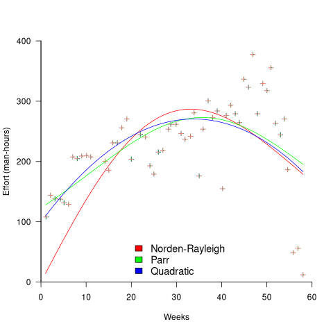
A variety of alternative forms for the quantity  have been proposed. An unpublished paper by H.M. Hubey discusses various possibilities.
Some researchers have fitted a selection of equations to manpower data, searching for the one that gives the best fit. The Gamma distribution is sometimes found to provide a better fit to a dataset. The argument for the Gamma distribution is not based on any theory, but purely on the basis of being the best fitting distribution, of those tested.
Putnam’s software equation debunked
The implementation of a project has a lifecycle that starts and finishes with zero people working on it. Between starting and finishing, the number of staff quickly grows to a peak before slowly declining. In a series of very hard to obtain papers during the early 1960s (chapter 5), Peter Norden created a large project staffing model described by the Rayleigh equation. This model was evangelized by Lawrence Putnam in the 1970s, who called it the Norden/Rayleigh model, while others sometimes now call it the Norden/Putnam, Putnam/Rayleigh, or some combination of names; Putnam’s papers can be hard to obtain.
The Norden/Rayleigh equation is: 
where:  is work completed,
  is total manpower over the lifespan of the project,
  ,
,  is time of maximum effort per unit time (i.e., the Norden/Rayleigh equation maximum value, which Putnam calls project development time), and
  is project elapsed time.
Norden’s model is only applicable to large projects (e.g., 2+ man-years), and Putnam points out that the staffing of small projects is usually a square wave, i.e., a number of staff are allocated at the start and this number remains the same until project completion.
As well as evangelizing Norden’s model, Putnam also created his own model; an equation connecting delivered lines of code, total manpower and project duration. The usually cited paper for this work is: “A General Empirical Solution to the Macro Software Sizing and Estimating Problem”, which can sometimes be found as a free download. I had always assumed that people did not take this model seriously, and it was not worth my time debunking it. The paper makes conjures hand-wavy connections between various equations which don’t seem to go anywhere, and eventually connects together a regression equation fitted to nine data points with an observation+assumption about another regression equation to create what Putnam calls the software equation:  , where
  is delivered source code statements, and
  is a constant.
I recently read a 2014 paper by Han Suelmann debunking Putnam’s software equation, which led me to question my assumption about people not using Putnam’s model. Google Scholar shows 1,411 citations, with 133 since 2020. It looks like the software equation is still being taken seriously (or researchers are citing it because everybody else does; a common practice).
Why isn’t Putnam’s software equation worth treating seriously?
First, Putnam’s derivation of the software equation reads like a just-so story based on a tiny amount of data, and second a larger independent dataset does not show the pattern seen in Putnam’s data.
The derivation of the software equation starts by defining productivity as the number of delivered source code statements divided by the total manpower consumed to produce them,  . Ok.
. Ok.
There is more certainty to a line fitted to a set of points that roughly follow a straight line, than to fit a line to points that follow a curve (because there are usually many ‘curve’ equations to choose from). The Norden/Rayleigh equation can be transformed to a form that is amenable to fitting a straight line, i.e., dividing by time and taking logs, as follows (which plugs in the value of  ):
):

Putnam noticed (or perhaps it was the authors of the cited prepublication paper “Software budgeting model” by G. E. P. Box and L. Pallesen, which I cannot locate a copy of) that when plotting  against
  : “If the number
  was small, it corresponded with easy systems; if the number was large, it corresponded with hard systems and appeared to fall in a range between these extremes.” Notice that in the screenshot of a figure from Putnam’s paper below, the y-axis is labelled “Difficulty”, not with the quantity actually plotted.
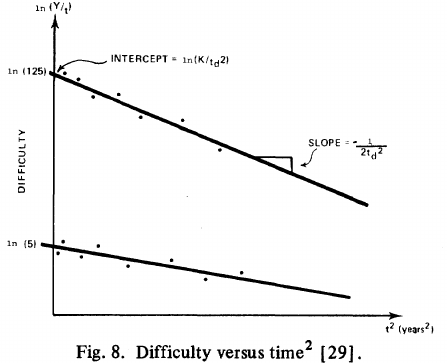
Based on an observation about easy/hard systems (it is never explained how easy/hard is measured) something called difficulty is defined to be:  . No explanation is given for dropping the log scaling, or the possibility that some other relationship might hold.
The screenshot below is of a figure from Putnam’s paper, which plots the values of  against
  for 13 projects. The fitted regression lines (the three lines are fitted using, 9, 2 and 2 points of the 13 projects) have the form
  , i.e.,
  (I extracted the points and fitted
  ; code+extracted data):
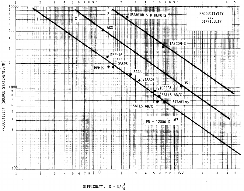
With a bit of algebra, the two equations:  and
and  , can be combined to create the software equation.
Yes, Putnam’s software equation was hand-waved into existence by plucking a “difficulty” component from an observation about the behavior of projects in a regression model and equating it to a regression line fitted to nine points.
Are the patterns seen by Putnam found in other projects?
In the 1987 paper “Time-Sensitive Cost Models in the Commercial MIS Environment” D. Ross Jeffery used data from 47 projects to investigate the effort/time relationships used by Putnam to derive his software equation.
The plot below, of log(Difficulty) vs log(Productivity), shows what appears to be a random scattering of points, confirmed by failing to fit a regression model (code+extracted data):

No. The patterns seen by Putnam are not present in these projects. I don’t think that the difference in application domain is relevant (Putnam’s projects were for Military systems and Jeffery’s are for commercial projects). Norden’s model is not specific to software projects.
Jeffery’s uses a regression model to find:  , the corresponding Putnam equation is:
  (the paper does not include the plot needed to extract the required data). The
  exponent might be claimed to be close enough, but the
  exponent is very different.
Jeffery’s paper includes a plot of  against
  , and the plot below shows the extracted data (44 points), plus fitted regression line (code+extracted data):
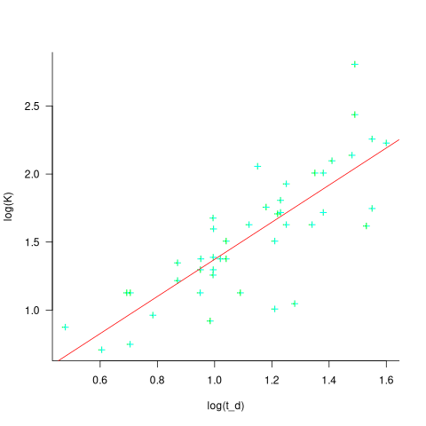
The regression line has the form  . This relationship further undermines assumptions made by Putnam, e.g., smaller systems are easier.
The Han Suelmann paper that triggered this post takes a very different approach to debunking Putnam’s model (he uses simulation to show that random data, drawn from a suitable distribution, can produce the patterns seen by Putnam).
Indented vs non-indented if-statements: performance difference
To non-developers discussions about the visual layout of source code can seem somewhat inconsequential. Layout probably ought to be inconsequential, being based on experimental studies that discovered how source should be visually organised to minimise the cognitive effort consumed by developers while processing it.
In practice software engineering is not evidence-based. There are two kinds of developers: those willing to defend to the death the layout they use, and those that have moved on.
In its simplest form visual layout involves indenting code some number of spaces from the left margin. Use of indentation has not always been widespread, and people wrote papers extolling the readability benefits of indenting code.
My experience with talking to developers about indentation is that they are heavily influenced by the indentation practices adopted by those around them when first learning a language. Layout habits from any prior language tend to last awhile, depending on the amount of time spent with the prior language.
As far as I know, I have had zero success arguing that the Gestalt principles of perception provide a useful framework for deciding between different code layouts.
The layout issue that attracts the most discussion is probably the indentation of if-statements. What, if any, is the evidence around this issue?
Developer indentation discussions focus on which indentation is better than the alternatives (whatever better might be). A more salient question would be the size of the developer performance difference, or is the difference large enough to care about?
Researchers have used several techniques for measuring difference in developer performance, including: code comprehension (i.e., number of correct answers to questions about the code they have just read), subjective ratings (i.e., how hard did the subjects find the task), and time to complete a task (e.g., modify source, find coding mistake).
The subjects have invariably been a small sample of undergraduates studying for a computing degree, so the usual caveats about applicability to professional developers apply.
Until 2023, the most detailed work I know of is a PhD thesis from 1974 studying the impact of mnemonic/meaningless variable names plus none/some indentation (experiments 1, 2 and 9), and a 1983 paper which compared subject performance with indentation of none and 2/4/6 spaces (contains summary data only). Both studies used small programs.
The 2023 paper Indentation in Source Code: A Randomized Control Trial on the Readability of Control Flows in Java Code with Large Effects by J. Morzeck, S. Hanenberg, O. Werger, and V. Gruhn measured the time taken by 20 subjects to answer 12 questions about the value printed by a randomly generated program containing a nested if-statement. The following shows an example without/with indentation (values were provided for i and j):
if (i != j) { if (i != j) { if (j > 10) { if (j > 10) { if (i < 10) { if (i < 10) { print (5); print (5); } else { } else { print (10); print (10); } } } else { } else { print (12); print (12); } } } else { } else { if (i < 10) { if (i < 10) { print (23); print (23); } else { } else { print (15); print (15); } } } } |
A fitted regression model found that the average response time of 122 seconds (yes, very slow) for non-indented code decreased to 44 seconds (not quite as slow) for indented code, i.e., about three times faster (code+data). This huge performance improvement is very different from most software engineering experiments where the largest effect is the between subjects performance, with learning producing the next largest effect.
Evidence that indentation is very effective, but nobody doubted this. There has been a follow-up study, more on that another time.
Employment in the software business: we know nothing
Tens of millions of people get paid to work on the creation and maintenance of software systems, by companies employing thousands of developers to those employing a single developer (in the UK there are almost 300K registered software companies; 5% of registered companies).
This huge ecosystem is almost completely ignored by the software engineering research community. Academics in computing/software are more interested in technical issue, and industry is an ecosystem they rarely interact with (some claim that student employment keeps them in contact with industry).
There are researchers in business and economics departments who study employment, e.g., careers, organization of workers and companies. The scientific study of work started at the beginning of the 1900s, originally focused on the manufacturing and included office work as that grew to employ a significant percentage of the workforce. Until recently, the percentage of the workforce employed to create/maintain software was not large enough to attract the attention of these researchers, and even now it’s often lumped together with other jobs that mostly involve some form of intellectual activity.
Employee related issues of interest to those involved in managing work on software systems are heavily influenced by the characteristics of the business ecosystem in which they work. The software driven business ecosystems are continually changing, with companies growing, merging and going bust as new markets emerge, grow, saturate, and sometime disappear. This constant change creates employment uncertainty, and lots of opportunities for competent people (creating a staff retention problem). For more stable industries, it’s possible for researchers to model employee start/promotion/leaving transitions using Markov models (example of ChatGPT 1o-preview solving a recurrence model of the staffing relationships in a 3-level employment hierarchy). The book “Stochastic Models for Social Processes” by D. J. Bartholomew gives a practical introduction to the use of Markov models for this kind of analysis.
The evolution and constant introduction of new technologies can make it difficult to find people with the appropriate skills. Companies may tune the wording of job adverts to give the impress of using ‘modern’ technologies, or post fake job adverts (to increase their attractiveness and suggest a feeling of growth), and people tune their CV to appeal to employers (some out right lie about their skills; many managers have told me that around 90% of applicants don’t have the primary skill sought by the employer). Well paid jobs can attract lots of applicants, filtering/interviewing can be an expensive process (not least because the same job title can denote different seniority in different companies). Matching CVs to job requirements sounds like the perfect use case for LLMs. I suspect that LLM tuning of CVs/adverts will just increase costs/uncertainty.
The constant churn of technologies forces employees to make decisions about whether to happily spend many years being well paid to become an expert in a niche with decreasing industry demand, or to invest in starting again as a non-expert doing something new (and initially less well paid).
What is the best to organize engineering employees at a company-wide scale? Matrix management was once the standard answer, but these days, scaled agile is a fashionable answer. An evidence-based answer will have to wait until the lawyers in a large organization allow somebody with the necessary skills access to the appropriate data.
With the contents of job sites being scraped, along with LinkedIn, I’m optimistic that some meaningful employment data will slowly become available. Will the analysis of this data uncover patterns of practical use (other than interesting blog posts) to employers/employees? We will have to wait and see.
Recent Comments