Archive
Christmas books for 2016
Here are couple of suggestions for books this Christmas. As always, the timing of the books I suggest is based on when they reach the top of the books-to-read pile, not when they were published.
“The Utopia of rules” by David Graeber (who also wrote the highly recommended “Debt : The First 5000 Years”). Full of eye opening insights into bureaucracy, how the ‘free’ world’s state apparatus came to have its current form and how various cultures have reacted to the imposition of bureaucratic rules. Very readable.
“How Apollo Flew to the Moon” by W. David Woods. This is a technical nuts-and-bolts story of how Apollo got to the moon and back. It is the best book I have every read on the subject, and as a teenager during the Apollo missions I read all the books I could find.
This year’s blog find was Scott Adams’ blog (yes, he of Dilbert fame). I had been watching Donald Trump’s rise for about a year and understood that almost everything he said was designed to appeal to a specific audience and the fact that it sounded crazy to those not in the target audience was irrelevant. I found Scott’s blog contained lots of interesting insights of the goings on in the US election; the insights into why Trump was saying the things he said have proved to be spot on.
For those of you interested in theoretical physics I ought to mention Backreaction (regular updates, primarily about gravity related topics) and Of Particular Significance (sporadic updates and primarily about particle physics)
Giving engineers the freedom to create a customer lock-in Cloud
The Cloud looks like the next dominant platform for hosting applications.
What can a Cloud vendor do to lock customers in to their fluffy part of the sky?
I think that Microsoft showed the way with their network server protocols (in my view this occurred because of the way things evolved, not though any cunning plan for world domination). The EU/Microsoft judgment required Microsoft to document and license their server protocols; the purpose was to allow third-parties to product Microsoft server plug-compatible products. I was an advisor to the Monitoring trustee entrusted with monitoring Microsoft’s compliance and got to spend over a year making sure the documents could be implemented.
Once most the protocol documents were available in a reasonably presentable state (Microsoft originally considered the source code to be the documentation and even offered it to the EU commission to satisfy the documentation requirement; they eventually hire a team of several hundred to produce prose specifications), two very large hurdles to third party implementation became apparent:
- the protocols were a tangled mess of interdependencies; 100% compatibility required implementing all of them (a huge upfront cost),
- the specification of the error behavior (i.e., what happens when something goes wrong) was minimal, e.g., when something unexpected occurs one of the errors in
windows.his returned (when I last checked, 10 years ago, this file contained over 30,000 identifiers).
Third party plugins for Microsoft server protocols are not economically viable (which is why I think Microsoft decided to make the documents public, they had nothing to loose and could claim to be open).
A dominant cloud provider has the benefit of size, they have a huge good-enough code base. A nimbler, smaller, competitor will be looking for ways to attract customers by offering a better service in some area, which means finding a smaller, stand-alone, niche where they can add value. Widespread use of Open Source means everybody gets to see and use most of the code. The way to stop smaller competitors gaining a foothold is to make sure that the code hangs together as a whole, with no relatively stand-alone components that can be easily replaced. Mutual interdependencies and complexity creates a huge barrier to new market entrants and is in the best interests of dominant vendors (yes it creates extra costs for them, but these are the price for detering competitors).
Engineers will create intendependencies between components and think nothing of it; who does not like easy solutions to problems and this one dependency will not hurt will it? Taking the long term view, and stopping engineers taking short cuts for short term gain, requires a lot of effort; who could fault a Cloud vendor for allowing mutual interdependencies and complexity to accumulate over time.
Error handling is a very important topic that rarely gets the attention it deserves, nobody likes to talk about the situation where things go wrong. Error handling is the iceberg of application development, while the code is often very mundane, its sheer volume (it can be 90% of the code in an application) creates a huge lock-in. The circumstances under which a system handles raises an error and the feasible recovery paths are rarely documented in any detail, it is something that developers working at the coal face learn by trial and error.
Any vendor looking to poach customers first needs to make sure they don’t raise any errors that the existing application does not handle and second any errors they do raise need to be solvable using the known recovery paths. Even if there is error handling information available to enable third-parties to duplicate responses, the requirement to duplicate severely hampers any attempt to improve on what already exists (apart from not raising the errors in the first place).
To create an environment for customer lock-in, Cloud vendors need to encourage engineers to keep doing what engineers love to do: adding new features and not worrying about existing spaghetti code.
Ability to remember code improves with experience
What mental abilities separate an expert from a beginner?
In the 1940s de Groot studied expertise in Chess. Players were shown a chess board containing various pieces and then asked to recall the locations of the pieces. When the location of the chess pieces was consistent with a likely game, experts significantly outperformed beginners in correct recall of piece location, but when the pieces were placed at random there was little difference in recall performance between experts and beginners. Also players having the rank of Master were able to reconstruct the positions almost perfectly after viewing the board for just 5 seconds; a recall performance that dropped off sharply with chess ranking.
The interpretation of these results (which have been duplicated in other areas) is that experts have learned how to process and organize information (in their field) as chunks, allowing them to meaningfully structure and interpret board positions; beginners don’t have this ability to organize information and are forced to remember individual pieces.
In 1981 McKeithen, Reitman, Rueter and Hirtle repeated this experiment, but this time using 31 lines of code and programmers of various skill levels. Subjects were given two minutes to study 31 lines of code, followed by three minutes to write (on a blank sheet of paper) all the code they could recall; this process was repeated five times (for the same code). The plot below shows the number of lines correctly recalled by experts (2,000+ hours programming experience), intermediates (just finished programming course) and beginners (just started programming course), left performance using ‘normal’ code and right is performance viewing code created by randomizing lines from ‘normal’ code; only the mean values in each category are available (code+data):
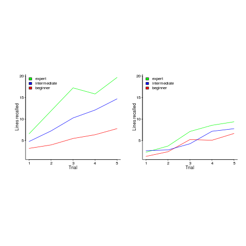
Experts start off remembering more than beginners and their performance improves faster with practice.
Compared to the Power law of practice (where experts should not get a lot better, but beginners should improve a lot), this technique is a much less time consuming way of telling if somebody is an expert or beginner; it also has the advantage of not requiring any application domain knowledge.
If you have 30 minutes to spare, why not test your ‘expertise’ on this code (the .c file, not the .R file that plotted the figure above). It’s 40 odd lines of C from the Linux kernel. I picked C because people who know C++, Java, PHP, etc should have no trouble using existing skills to remember it. What to do:
- You need five blank sheets of paper, a pen, a timer and a way of viewing/not viewing the code,
- view the code for 2 minutes,
- spend 3 minutes writing down what you remember on a clean sheet of paper,
- repeat until done 5 times.
Count how many lines you correctly wrote down for each iteration (let’s not get too fussed about exact indentation when comparing) and send these counts to me (derek at the primary domain used for this blog), plus some basic information on your experience (say years coding in language X, years in Y). It’s anonymous, so don’t include any identifying information.
I will wait a few weeks and then write up the data o this blog, as well as sharing the data.
Update: The first bug in the experiment has been reported. It takes longer than 3 minutes to write out all the code. Options are to stick with the 3 minutes or to spend more time writing. I will leave the choice up to you. In a test situation, maximum time is likely to be fixed, but if you have the time and want to find out how much you remember, go for it.
Power law of practice in software implementation
People get better with practice. The power law of practice specifies 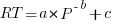 , where:
  is the response time,
  the amount of practice and
  ,
,  and
and  are constants. However, sometimes an exponential equation is a better fit for to the data:
 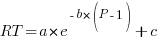 . There are theoretical reasons for liking a power law (e.g., it can be derived from the chunking of information), but it is difficult to argue with the exponential fitting so much data better than a power law.
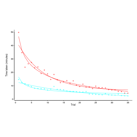
The plot below, from a study by Alteneder, shows the time taken to solve the same jig-saw puzzle, for 35 trials (red); followed by a two week pause and another 35 trials (in blue; if anybody else wants to try this, a dedicated weekend should be long enough to complete over 20 trials). The lines are fitted power law and exponential equations (code+data). Can you tell which is which?
To find out if the same behavior occurs with software we need data on developers implementing the identical applications multiple times. I know of two experiments where the same application has been implemented multiple times by the same people, and where the data is available. Please let me know if you know of any others.
Zislis timed himself implementing 12 algorithms from the CACM collection in each of three languages, iterating four times (my copy came from the Purdue library, which as I write this is not listing the report). The large number of different programs implemented, coupled with the use of multiple languages, makes it difficult to separate out learning effects.
Lui and Chan ran an experiment where 24 developers (8 pairs {pair programming} and 8 singles) implemented the same application four times. The plot below shows the time taken to complete each implementation (singles top, pairs bottom, with black cross showing predictions made by a power law fit).
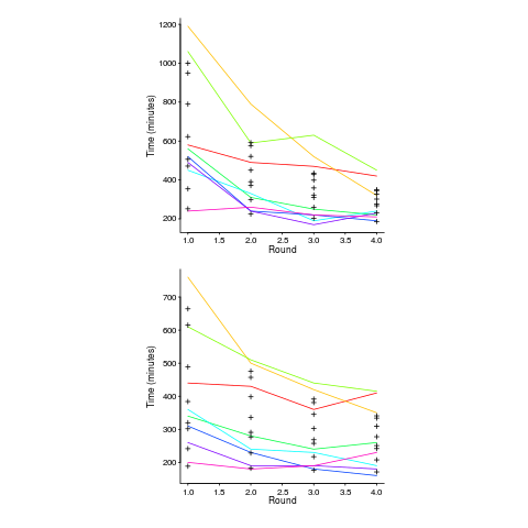
Different subjects start the experiment with different amounts of ability and past experience. Before starting, subjects took a multiple choice test of their knowledge. If we take the results of this test as a proxy for the ability/knowledge at the start of the experiment, then the power law equation becomes (a similar modification can be made to the exponential equation):

That is, the test score is treated as equivalent to performing some number of rounds of implementation). A power law is a better fit than exponential to this data (code+data); the fit captures the general shape, but misses lots of what look like important details.
The experiment was run over successive weekends. So there was opportunity for some forgetting to occur during the week days, and the amount forgotten will vary between people. It is easy to think of other issues that could have influenced subject performance.
This experiment must rank as one of the most interesting software engineering experiments performed to date.
Uncertainty in data causes inconsistent models to be fitted
Does software development benefit from economies of scale, or are there diseconomies of scale?
This question is often expressed using the equation:  . If is less than one there are economies of scale, greater than one there are diseconomies of scale. Why choose this formula? Plotting project effort against project size, using logs scales, produces a series of points that can be sort-of reasonably fitted by a straight line; such a line has the form specified by this equation.
Over the last 40 years, fitting a collection of points to the above equation has become something of a rite of passage for new researchers in software cost estimation; values for have ranged from 0.6 to 1.5 (not a good sign that things are going to stabilize on an agreed value).
This article is about the analysis of this kind of data, in particular a characteristic of the fitted regression models that has been baffling many researchers; why is it that the model fitted using the equation is not consistent with the model fitted using  , using the same data. Basic algebra requires that the equality
  be true, but in practice there can be large differences.
The data used is Data set B from the paper Software Effort Estimation by Analogy and Regression Toward the Mean (I cannot find a pdf online at the moment; Code+data). Another dataset is COCOMO 81, which I analysed earlier this year (it had this and other problems).
The difference between and  is a result of what most regression modeling algorithms are trying to do; they are trying to minimise an error metric that involves just one variable, the response variable.
In the plot below left a straight line regression has been fitted to some Effort/Size data, with all of the error assumed to exist in the  values (dotted red lines show the residual for each data point). The plot on the right is another straight line fit, but this time the error is assumed to be in the
  values (dotted green lines show the residual for each data point, with red line from the left plot drawn for reference). Effort is measured in hours and Size in function points, both scales show the
  of the actual value.
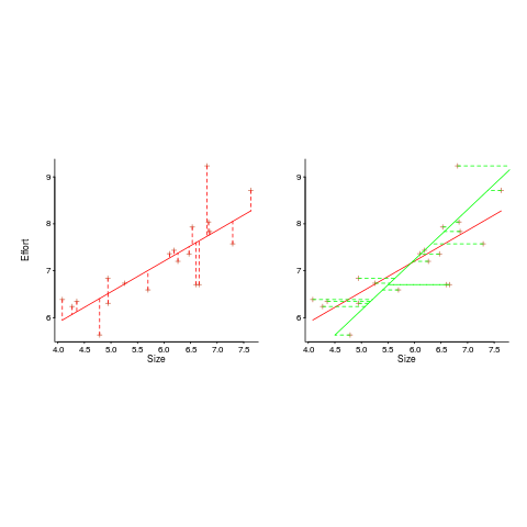
Regression works by assuming that there is NO uncertainty/error in the explanatory variable(s), it is ALL assumed to exist in the response variable. Depending on which variable fills which role, slightly different lines are fitted (or in this case noticeably different lines).
Does this technical stuff really make a difference? If the measurement points are close to the fitted line (like this case), the difference is small enough to ignore. But when measurements are more scattered, the difference may be too large to ignore. In the above case, one fitted model says there are economies of scale (i.e.,  ) and the other model says the opposite (i.e.,
  , diseconomies of scale).
There are several ways of resolving this inconsistency:
- conclude that the data contains too much noise to sensibly fit a a straight line model (I think that after removing a couple of influential observations, a quadratic equation might do a reasonable job; I know this goes against 40 years of existing practice of do what everybody else does…),
- obtain information about other important project characteristics and fit a more sophisticated model (characteristics of one kind or another are causing the variation seen in the measurements). At the moment information is being used to explain all of the variance in the data, which cannot be done in a consistent way,
- fit a model that supports uncertainty/error in all variables. For these measurements there is uncertainty/error in both and ; writing the same software using the same group of people is likely to have produced slightly different Effort/Size values.
There are regression modeling techniques that assume there is uncertainty/error in all variables. These are straight forward to use when all variables are measured using the same units (e.g., miles, kilogram, etc), but otherwise require the user to figure out and specify to the model building process how much uncertainty/error to attribute to each variable.
In my Empirical Software Engineering book I recommend using simex. This package has the advantage that regression models can be built using existing techniques and then ‘retrofitted’ with a given amount of standard deviation in specific explanatory variables. In the code+data for this problem I assumed 10% measurement uncertainty, a number picked out of thin air to sound plausible (its impact is to fit a line midway between the two extremes seen in the right plot above).
Pre-Internet era books that have not yet been bettered
It is a surprise to some that there are books written before the arrival of the Internet (say 1995) that have not yet been improved on. The list below is based on books I own and my thinking that nothing better has been published on that topic may be due to ignorance on my part or personal bias. Suggestions and comments welcome.
Before the Internet the only way to find new and interesting books was to visit a large book shop. In my case these were Foyles, Dillons (both in central London) and Computer Literacy (in Silicon valley).
Foyles was the most interesting shop to visit. Its owner was somewhat eccentric, books were grouped by publisher and within these subgroups alphabetic by author, and they stocked one of everything (many decades before Amazon’s claim to fame of stocking the long tail, but unlike Amazon they did not have more than one of the popular books). The lighting was minimal, every available space was piled with books (being tall was necessary to reach some books), credit card payment had to be transacted through a small window in the basement reached via creaky stairs or a 1930’s lift. A visit to the computer section at Foyles, which back in the day held more computer books than any other shop I have ever visited, was an afternoon’s experience (the end result of tight fisted management, not modern customer experience design), including the train journey home with a bundle of interesting books. Today’s Folyes has sensible lighting, a Coffee shop and 10% of the computer books it used to have.
When they can be found, these golden oldies are often available for less than the cost of the postage. Sometimes there are republished versions that are cheaper/more expensive. All of the books below were originally published before 1995. I have listed the ISBN for the first edition when there is a second edition (it can be difficult to get Amazon to list first editions when later editions are available).
“Chaos and Fractals” by Peitgen, Jürgens and Saupe ISBN 0387979034. A very enjoyable months reading. A second edition came out around 2004, but does not look to be that different from the 1992 version.
“The Terrible Truth About Lawyers” by Mark H. McCormack, ISBN 0002178699. Very readable explanation of how to deal with lawyers.
“Understanding Comics: The Invisible Art” by Scott McCloud. A must read for anybody interested in producing code that is easy to understand.
“C: A Reference Manual” by Samuel P. Harbison and Guy L. Steele Jr, ISBN 0-13-110008-4. Get the first edition from 1984, subsequent editions just got worse and worse.
“NTC’s New Japanese-English Character Dictionary” by Jack Halpern, ISBN 0844284343. If you love reading dictionaries you will love this.
“Data processing technology and economics” by Montgomery Phister. Technical details covering everything you ever wanted to know about the world of 1960’s computers; a bit of a specialist interest, this one.
I ought to mention “Godel, Escher, Bach” by D. Hofstadter, which I never rated but lots of other people enjoyed.
Producing software for money and/or recognition
In the commercial environment money makes the world go around, while in academia recognition (e.g., number of times your work is cited, being fawned over at conferences, impressive job titles) is the coin of the realm (there are a few odd balls who do it out of love for the subject or a desire to understand how things work, but modern academia is a large bureaucracy whose primary carrot is recognition).
There is an incentive problem for those writing software in academia; software does not attract much, if any, recognition.
Does the lack of recognition for writing software matter? Surely what counts are the research results, not the tools used to get there (be they writing software or doing mathematics).
A recent paper bemoans the lack of recognition for the development of Python packages for Astronomy researchers. Well, its too late now, they have written the software and everybody gets to make perfect copies for free.
What the authors of Astropy want, is for researchers who use this software to include a citation to it in any published papers. Do all 162 authors deserve equal credit? If a couple of people add a new package, should they get a separate citation? What if a new group of people take over maintenance, when should the citation switch over from the old authors/maintainers to the new ones? These are a couple of the thorny questions that need to be answered.
R is perhaps the most widely used academic developed software ecosystem. A small dedicated group of people has invested a lot of their time over many years to make something special. A lot more people have invested effort to create a wide variety of add-on packages.
The base R library includes the citation function, which returns the BibTeX information for a given package; ready to be added to a research papers work flow.
Both commercial and academic producers need to periodically create new versions to keep ahead of the competition, attract more customers and obtain income. While they both produce software to obtain ‘income’, commercial and academic software systems have different incentives when it comes to support for end users of the software.
Keeping existing customers happy is the way to get them to pay for upgrades and this means maintaining compatibility with what went before. Managers in commercial companies make sure that developers don’t break backwards compatibility (developers hate having to code around what went before and would love to throw it all away).
In the academic world it does not matter whether end users upgrade, as long as they cite the package, the version used is irrelevant; so there is a lot less pressure to keep backwards compatibility. Academics are supposed to create new stuff, they are researchers after all, so the incentives are pushing them to create brand new packages/systems to be seen as doing new stuff (and obtain a whole new round of citations). A good example is Hadley Wickham, who has created some great R packages, who seems to be continually moving on, e.g., reshape -> reshape2 -> tidyr (which is what any good academic is supposed to do).
The run-time performance of a system is something end users always complain about, but often get used to. The reason is invariably that there is little or no incentive to address this issue (for both commercial and academic systems). Microsoft Windows is slower than it need be and the R interpreter could go a lot faster (the design of the interpreter looks like something out of the 1980s; I’m seeing a lot of packages in R only, so the idea that R programs spend all their time executing in C/Fortran libraries may be out of date. Where is the incentive to use post-2000 designs?)
How many new versions of a software package can be produced before enough people stop being willing to pay for an update? How many different packages solving roughly the same problem can academics produce?
I don’t think producing new packages for income has a long term future.
Software architect is an illegal job title in the UK
If you are working in the UK with the job title “software architect”, or styling yourself as such, you are breaking the law. Yes, you are committing an offense under: Architects Act 1997 Part IV Section 20. In particular: “(1) A person shall not practise or carry on business under any name, style or title containing the word “architect” unless he is a person registered [F1 in Part 1 of the Register].”
The Architecture Registration Board are happy to take £142 off you, ever year, for the privilege of using architect in your job title. There is also the matter of a Part 3 examination; don’t know what that is.
If you really do like the word architect in your job title and don’t want to pay £142 a year, you could move into another line of business: “(2) Subsection (1) does not prevent any use of the designation “naval architect”, “landscape architect” or “golf-course architect”.” I am assuming that the he in the wording also applies to she‘s and that a sex change will not help.
Do building architects care? I suspect not. Are the police going to do anything about it? Well, if they don’t like you and are looking for some way of hauling you before the courts, the fine is not that bad.
A signature for the “embeddedness” of source code and developers?
Patterns in the use of source code can tell us a lot about the people who wrote the code, the characteristics of the hardware it runs on and what the application is all about.
Often the pattern of usage needs a lot of work to understand and many remain completely baffling, but every now and again the forces driving a pattern leap off the page. One such pattern is visible in the plot below; data courtesy of Jacob Engblom and the cbook data is from my C book (assuming you know something about the nitty gritty of embedded software development). It shows the percentage of functions defined to have a given number of parameters:
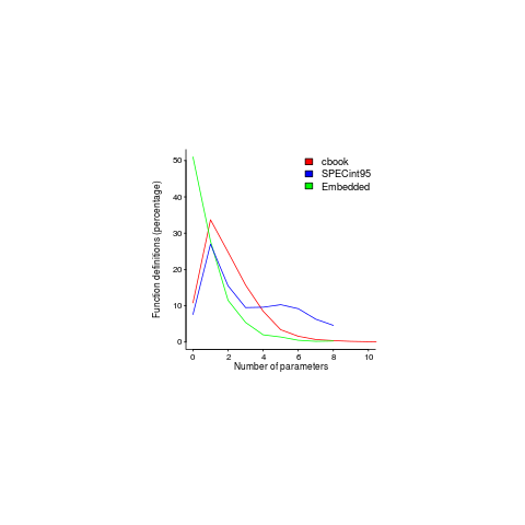
Embedded software has to run in very constrained environments. The hardware is often mass produced and saving a penny per device can add up to big savings, so the cheapest processor is chosen and populated with the smallest possible memory; developers have to work with what they are given. Power consumption may be down below one watt, so clock speeds are closer to 1 MHz than 1 GHz.
Parameter passing is a relatively expensive operation and there are major savings, relatively speaking, to be had by using global variables. Experienced embedded developers know this and this plot is telling us that they are acting on this knowledge.
The following are two ways of interpreting the embedded data (I cannot think of any others that make sense):
- the time/resource critical functions use globals rather than parameters and all the other functions are written more or less the same as in a non-embedded environment. In statistical terms this behavior is described by a zero-inflated model,
- there is pressure on the developer to reduce the number of parameters in all function definitions.
This data contains counts, so a Poisson distribution is the obvious candidate for our model.
My attempts to fit a zero-inflated model failed miserably (code+data). A basic Poisson distribution fitted everything reasonably well (let’s ignore that tiresome bump in the blue line); plus signs are the predictions made from each fitted model.
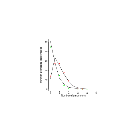
For desktop developers, the distribution of function definitions having a given number of parameters follows a Poisson distribution with a λ of 2, while for embedded developers λ is 0.8.
What about values of λ between 0.8 and 2; perhaps the λ of a project’s, or developer’s, code parameter count can be used as an indicator of ’embeddedness’?
What is needed to parameter count data from a range of 4-bit, 8-bit and 16-bit systems and measurements of developers who have been working in the field for, say, 4, 8, 16 years. Please let me know.
The data is from a Masters thesis written in 1999, is it still relevant today? Have modern companies become kinder to developers and stopped making their life so hard by saving pennies when building mass produced products; are modern low-power devices being used so values can be passed via parameters rather than via globals, or are they being used for applications where even less power is available?
One difference from 20 years ago is that embedded devices are more mainstream, easier to get hold of and sales opportunities abound. This availability creates an environment where developers with a desktop development mentality (which developers new to embedded always seem to have had) don’t get to learn about the overheads of parameter passing.
Have compilers gotten better at reducing the function parameter overhead? The most obvious optimization is inlining a function at the point of call. If the function is only called once, this works fine, with multiple calls the generated code can get larger (one of the things we are trying to avoid). I don’t have any reliable data on modern compiler performance int his area, but then I have not looked hard. Pointers to benchmarks welcome.
Does embedded software have any other signatures that differentiate it from desktop software (other than the obvious one of specifying address in definitions of global variables)? Suggestions welcome.
Fortran 2008 Standard has been updated
An updated version of ISO/IEC 1539-1 Information technology — Programming languages — Fortran — Part 1: Base language has just been published. So what has JTC1/SC22/WG5 been up to?
This latest document is bug a release of the 2010 standard, known as Fortran 2008 (because the ANSI Standard from which the ISO Standard was derived, sed -e "s/ANSI/ISO/g" -e "s/National/International/g", was published in 2008) and incorporates all the published corrigenda. I must have been busy in 2008, because I did not look to see what had changed.
Actually the document I am looking at is the British Standard. BSI don’t bother with sed, they just glue a BSI Standards Publication page on the front and add BS to the name, i.e., BS ISO/IEC 1539-1:2010.
The interesting stuff is in Annex B, “Deleted and obsolescent features” (the new features are Fortranized versions of languages features you have probable seen elsewhere).
Programming language committees are known for issuing dire warnings that various language features are obsolescent and likely to be removed in a future revision of the standard, but actually removing anything is another matter.
Well, the Fortran committee have gone and deleted six features! Why wasn’t this on the news? Did the committee foresee the 2008 financial crisis and decide to sneak out the deletions while people were looking elsewhere?
What constructs cannot now appear in conforming Fortran programs?
- “Real and double precision DO variables. .. A similar result can be achieved by using a DO construct with no loop control and the appropriate exit test.”
What other languages call a for-loop, Fortran calls a DO loop. So loop control variables can no longer have a floating-point type.
- “Branching to an END IF statement from outside its block.”
An if-statement is terminated by the token sequence
END IF, which may have an optional label. It is no longer possible toGOTOthat label from outside the block of the if-statement. You are going to have to label the statement after it. - “PAUSE statement.”
This statement dates from the days when a computer (singular, not plural) had its own air-conditioned room and a team of operators to tend its every need. A
PAUSEstatement would cause a message to appear on the operators’ console and somebody would be dispatched to check the printer was switched on and had paper, or some such thing, and they would then resume execution of the paused program.I think WG5 has not seen the future here. Isn’t the
PAUSEstatement needed again for cloud computing? I’m sure that Amazon would be happy to quote a price for having an operator respond to aPAUSEstatement. - “ASSIGN and assigned GO TO statements and assigned format specifiers.”
No more assigning labels to variables and GOTOing them, as a means of leaping around 1,000 line functions. This modern programming practice stuff is a real killjoy.
- “H edit descriptor.”
First programmers stopped using punched cards and now the H edit descriptor have been removed from Fortran; Herman Hollerith no longer touches the life of working programmers.
In the good old days real programmers wrote
11HHello World. Using quote delimiters for string literals is for pansies. - “Vertical format control. … There was no standard way to detect whether output to a unit resulted in this vertical format control, and no way to specify that it should be applied; this has been deleted. The effect can be achieved by post-processing a formatted file.”
Don’t panic, C still supports the
\vescape sequence.
Recent Comments