The Shape of Code

Is it possible to reliably estimate the elapsed time that a multi-person Open source project spends under major active development, once it has been running for a year or so, and attracted some developers?

The paper Project Life Cycles in Open-Source Software by Das, Ieroshenko, Jain, Qiu, Chin, and Granger fits a Bass diffusion model to the number of monthly developers contributing to a project, and then extrapolates the fitted equation into the future. Is the Bass model a good fit to this kind of data, and how reliable might its prediction be?

What first caught my attention in this paper was the appearance of the sech function (i.e., the hyperbolic secant: ) in the derived formula. The only other place I have encountered this function in software engineering is the Parr model of project staffing distribution, e.g., effort in hours per week. What’s more, both instances involve sech squared, i.e., .

Is this use of a coincidence, or is there an interesting connection? Let’s look at the paper.

The Bass diffusion model, or just Bass model, assumes that the number of people buying a new product is controlled by two factors: 1) independents who have a constant probability, , of buying it, and 2) imitators whose probability of purchase depends on times the number of existing users of the product (see section 3.6.3 of my book). The Bass model has been extended to handle successive, overlapping generations of a product, e.g., IBM mainframes.

I have not seen the Bass model applied to software lifecycles before (a quick search found a 2014 paper using it to model the time-evolution of package dependencies).

The authors of the new paper introduced sech by normalising two variables in the Bass equation:
Time, is normalised by dividing by time of peak development, , and number of developers, , is normalised by dividing by peak number of developers, , giving:
, where , and . It’s not possible to fit this equation to project data because the peak development values are not known (or might not yet have been reached).

The equation in the Parr model is: , where the values of and are obtained by fitting a regression model to project data. The derivation of the Parr model assumes that as project implementation progresses, new problems that need to be solved are discovered (e.g., features to be implemented), an existing problem can spawn at most two new subproblems, and the number of new problems discovered at any time is proportional to the number of remaining problems (cannot find an online version of “An alternative to the Rayleigh curve model for software development effort”).

A connection can be made between the Bass and Parr models by equating the number of developers contributing with the number of problems to be solved, with contributors treated as independents or imitators. The opportunities for potential contributors are likely to increase as a project starts up and then, for some projects decrease (projects such as the Linux kernel just keep on going). The problem implemented by a developer could spawn more than two subproblems.

In practice most of the implementation work on an Open source project is done by a small percentage of developers, with some projects dieing after loosing a few core developers. There is also the issue of the same person contributing using multiple identities.

One method for checking how well a model predicts future measurements is to compare the equations fitted using all the monthly data and, say, the first 75% months. The extent to which both fitted equations agree provides an indication of the likely accuracy of currently unknown future values. The Das et al paper fits the Bass model to the monthly contributor data from 23 projects. The plot below shows the number of monthly developers for numpy (since the project started), along with two fitted Bass models, one for all the data and the other for the first 75% of the data (code+data):

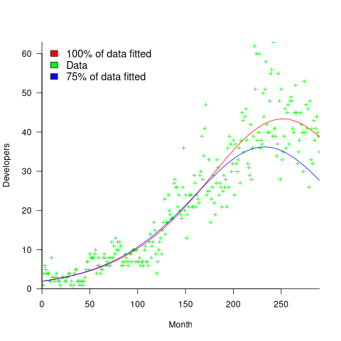
The example project used in the paper has a closer agreement between the two fitted equations, and some of the other projects have much less agreement. The Bass models assumes that monthly contributions are primarily driven by two factors. In practice there could be many other factors driving developer involvement in a project.

Predicting when a project is likely to stop growing is a notoriously difficult problem. Fitting a logistic equation to the growth in lines of code is another example of a model fitting the pattern present in the underlying equation (which flattens off).

It’s possible that weighting developer contribution by the amount of functionality (not lines of code) will produce a closer agreement between theory and practice.

The Putnam project staffing model predates the Parr mode, and later research found that the Putnam model was also a poor predictor of project durations. Both the Parr and Putnam equations can be derived using hazard analysis.

Applying the Bass multi-product generation model to software evolution is now on my to-do list, e.g., use of PHP versions.