Archive
Will incorrect answers be biased towards one arm of an if-statement?
Sometimes it is possible to deduce which arm of a nested if-statement will be executed by looking at the form of the conditional expression in the outer if-statement, as in:
if ((L < M) && (M < H)) if (L < H) ; // Execution always end up here else ; // dead code |
but not in:
if ((L > M) && (M < H)) if (L < H) ; // Could end up here else ; // or here |
I ran an experiment at the 2012 ACCU conference where subjects saw nested if-statements like those above and had to specify which arm of the nested if-statement would be executed.
Sometimes subjects gave an answer specifying one arm when in fact both arms are possible. Now dear reader, do you think these incorrect answers will specify the then arm 50% of the time and the else arm 50% or do you think that that incorrect answers will more often specify one particular arm?
Of course I should have thought about this before I started to analyse the data, but this question is unrelated to the subject of the experiment and has only just cropped up because of the unexpectedly high percentage of this kind of incorrect answer. I had an idea what the answer would be but did not stop and think about relative percentages, rushing off to write a few lines of code to print the actual totals, so now my mind is polluted by knowing the answer (well at least for one group of subjects in one experiment).
Why does this “one arm preference” issue matter? The Bayesians out there will insist that the expected distribution (the prior in Bayesian terminology) of incorrectly chosen arms be factored in to the calculation of the probability of getting the numbers seen in the results. The paper Belgian euro coins: 140 heads in 250 tosses – suspicious? gives a succinct summary of the possibilities.
So I have decided to appeal to my experienced readership, yes YOU!
For those questions where the actual execution cannot be predicted in advance, from knowledge of the relative values of variables appearing in the outer if-statement, when an incorrect answer is given should the analysis assume:
- a 50/50 split of incorrect answers between each arm, or
- subjects are more likely to pick one arm; please specify a percentage breakdown between arms.
No pressure, but the submission deadline is very late tomorrow.
The results from the whole experiment will get written up here in future posts.
Update (three days later): Nobody was willing to stick their head above the parapet 🙁
There were 69 correct answers and 16 incorrect answers to questions whose answer was “both arm”. Ten of those incorrect answers specified the ‘then’ arm and 6 the ‘else’; my gut feeling was that there should be even more ‘then’ answers. If there was no “first arm” there is an equal probability of a subject’s incorrect answer appearing in either arm; in this case the probability of a 10/6 split is 12% (so my gut feeling was just hunger pangs after all).
Will programming languages now have to follow ISO fast-track rules?
A while back I wrote about how updated versions of ECMAscript (i.e., the Standard for Javascript) had twice been fast tracked to replace an existing ISO Standard, however the ISO rules require that once a document becomes one of its standards all future work be done using the ISO process (i.e., you only supposed to get the one original fast track and then you have to get at least half a dozen countries to say they will actively participate in ongoing work). Thirteen years after I asked why it was being allowed to happen (as I recall I only raised the issue because I thought I had misunderstood the rules, not because I had a burning desire to enforce them) the issue has suddenly sprung to life (we are talking Standard’s world ‘sudden’ here), with a question being raised at the last SC22 meeting and a more detailed one being prepared by BSI for the next meeting (they occur once per year).
The Elephant in the room here is ISO/IEC 29500:2008, not a programming language but Microsoft’s Office Open XML; there was quite a bit of fuss when this was fast tracked.
If the ISO rules on one-time only use of the fast track process was limited to programming languages I imagine the bureaucrats in Geneva would probably never get to hear about it (SC22 would probably conclude that there was not enough interest in the various documents outside of the submitting country to form an active ISO working group; so leave well alone).
ISO sells over 19,000 standards and has better things to do than spend time on the goings on in an unfashionable part of the galaxy, unless, that is, it has the potential to generate lots of fuss that undermines credibility.
Will Microsoft try to fast track an updated version of ISO 29500? I don’t even know if they are updating it. The possibility that ISO 29500 might be updated and submitted for fast track will make it hard for SC22 to agree to any future fast-track updates to existing ISO Standards it is responsible for.
The following is a list of documents that have been fast tracked to become an ISO Standard:
ECMAScript:
ECMA-262 (1st edn) = ISO 16262:1998
ECMA-262 (3rd edn) = ISO 16262:1999
ECMA-262 (5th edn) = ISO 16262:2011

C#:
ECMA-334 (2nd edn) = ISO 23270:2003
ECMA-334 (4th edn) = ISO 23270:2006

CLI:
ECMA-335 (2nd edn) = ISO 23271:2003
ECMA-335 (6th edn) = ISO 23271:2012

ECMA standards fast-tracked to ISO and not yet revised:
ECMA-149 PCTE part 1 = ISO 13719-1:1998
ECMA-158 PCTE part 2 = ISO 13719-2:1998
ECMA-162 PCTE part 3 = ISO 13719-3:1998
ECMA-230 PCTE IDL binding = ISO 13719-4:1998
ECMA-367 EIFFEL = ISO 25436:2006
ECMA-372 C++/CLI -> DIS 26926; failed DIS ballot and project cancelled

Replaced rather than revised under JTC1 rules:
CHILL (from CCITT): ISO standards 9496:1989, 9496:1995, 9496:1998, 9496:2003
MUMPS/M (from Mass Gen Hospital/ANSI): ISO standards 11756:1992, 11756:1999

Non-ECMA documents fast-tracked through ISO and not yet revised:
FORTH (from FORTH Inc): ISO 15145:1997
JEFF (from J consortium): ISO 20970:2002
Ruby (from Japanese Industrial Standards Committee): ISO/IEC 30170:2012
Popularity of Open source Operating systems over time
Surveys of operating system usage trends are regularly published and we get to read about how the various Microsoft products are doing and the onward progress of mobile OSs; sometimes Linux gets an entry at the bottom of the list, sometimes it is just ‘others’ and sometimes it is both.
Operating systems are pervasive and a variety of groups actively track reported faults in order to issue warnings to the public; the volume of OS fault informations available makes it an obvious candidate for testing fault prediction models (e.g., how many faults will occur in a given period of time). A very interesting fault history analysis of OpenBSD in a paper by Ozment and Schechter recently caught my eye and I wondered if the fault time-line could be explained by the time-line of OpenBSD usage (e.g., more users more faults reported). While collecting OS usage information is not the primary goal for me I thought people would be interested in what I have found out and in particular to share the OS usage data I have managed to obtain.
How might operating system usage be measured? Analyzing web server logs is an obvious candidate method; when a web browser requests information many web servers write information about the request to a log file and this information sometimes includes the name of the operating system on which the browser is running.
Other sources of information include items sold (licenses in Microsoft’s case, CDs/DVD’s for Open source or perhaps books {but book sales tend not to be reported in the way programming language book sales are reported}) and job adverts.
For my time-line analysis I needed OpenBSD usage information between 1998 and 2005.
The best source of information I found, by far, of Open source OS usage derived from server logs (around 138 million Open source specific entries) is that provided by Distrowatch who count over 700 different distributions as far back as 2002. What is more Ladislav Bodnar the founder and executive editor of DistroWatch was happy to run a script I sent him to extract the count data I was interested in (I am not duplicating Distrowatch’s popularity lists here, just providing the 14 day totals for OS count data). Some analysis of this data below.
As luck would have it I recently read a paper by Diomidis Spinellis which had used server log data to estimate the adoption of Open Source within organizations. Diomidis researches Open source and was willing to run a script I wrote to extract the User Agent string from the 278 million records he had (unfortunately I cannot make this public because it might contain personal information such as email addresses, just the monthly totals for OS count data, tar file of all the scripts I used to process this raw log data; the script to try on your own logs is countos.sh).
My attempt to extract OS names from the list of User Agent strings Diomidis sent me (67% of of the original log entries did contain a User Agent string) provides some insight into the reliability of this approach to counting usage (getos.awk is the script to try on the strings extracted with the earlier script). There is no generally agreed standard for:
- what information should be present; 6% of UA strings contained no OS name that I knew (this excludes those entries that were obviously robots/crawlers/spiders/etc),
- the character string used to specify a given OS or a distribution; the only option is to match a known list of names (OS names used by Distrowatch,
missos.awkis the tar file script to print out any string not containing a specified list of OS names, the Wikipedia List of operating systems article), - quality assurance; some people cannot spell ‘windows’ correctly and even though the source is now available I don’t think anybody uses CP/M to access the web (at least 91 strings,
 %, would not have passed).
Ladislav Bodnar thinks that log entries from the same IP addresses should only be counted once per day per OS name. I agree that this approach is much better than ignoring address information; why should a person who makes 10 accesses be counted 10 times, a person who makes one access is only counted once. It is possible that two or more separate machines running the same OS are accessing the Internet through a common gateway that results in them having the IP address from an external server’s point of view; this possibility means that the Distrowatch data undercounts the unique accesses (not a serious problem if most visitors have direct Internet access rather than through a corporate network).
The Distrowatch data includes counts for all IP address and from 13 May 2004 onwards unique IP address per day per OS. The mean ratio between these two values, summed over all OS counts within 14 day periods, is 1.9 (standard deviation 0.08) and the Pearson correlation coefficient between them is 0.987 (95% confidence interval is 0.984 to 0.990), i.e., almost perfect correlation.
The Spinellis data ignores IP address information (I got this dataset first, and have already spent too much time collecting to do more data extraction) and has 10 million UA strings containing Open source OS names (6% of all OS names matched).
How representative are the Distrowatch and Spinellis data? The data is as representative of the general OS population as the visitors recorded in the respective server logs are representative of OS usage. The plot below shows the percentage of visitors to Distrowatch that use Ubuntu, Suse, Redhat. Why does Redhat, a very large company in the Open source world, have such a low percentage compared to Ubuntu? I imagine because Redhat customers get their updates from Redhat and don’t see a need to visit sites such as Distrowatch; a similar argument can be applied to Suse. Perhaps the Distrowatch data underestimates those distributions that have well known websites and users who have no interest in other distributions. I have not done much analysis of the Spinellis data.
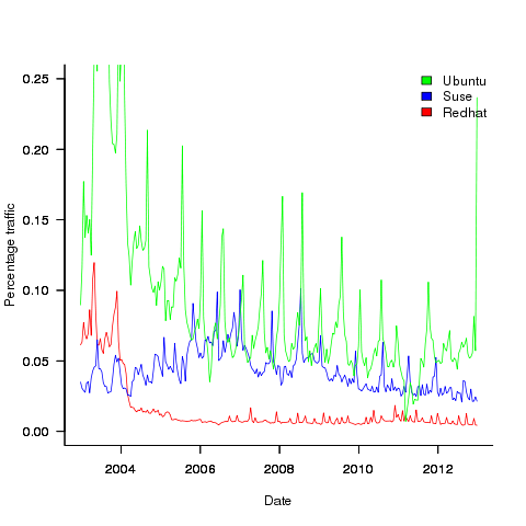
Presumably the spikes in usage occur around releases of new versions, I have not checked.
For my analysis I am interested in relative change over time, which means that representativeness and not knowing the absolute number of OSs in use is not a problem. Researchers interested in a representative sample or estimating the total number of OSs in use are going to need a wider selection of data; they might be interested in the following OS usage information I managed to find (yes I know about Netcraft, they charge money for detailed data and I have not checked what the Wayback Machine has on file):
- Wikimedia has OS count information back to 2009. Going forward this is a source of log data to rival Distrowatch’s, but the author of the scripts probably ought to update the list of OS names matched against,
- w3schools has good summary data for many months going back to 2003,
- statcounter has good summary data (daily, weekly, monthly) going back to 2008,
- TheCounter.com had data from 2000 to 2009 (csv file containing counts obtained from Wayback Machine).
If any reader has or knows anybody who has detailed OS usage data please consider sharing it with everybody.
Only compiler vendor customers, not its users, count
The hardest thing about working on compilers is getting somebody to pay you to do it (its a close run race against having the cpu instructions chop and change under you during initial development, but that’s another story). The major shift of compiler vendor business model from proprietary to open source has significant implications for users of compilers. Note I said user not customer, only one of them pays money. Under the commercial model there was usually a very direct connection between compiler user and customer (even in large organizations users rather than the manager who makes the purchase decision are often regarded by vendors as the customer), while under the Open source model most users are not customers (paying money for a distribution does not make you a customer of the people maintaining the compiler who probably don’t receive any of the money you spent).
Like all good businesses compiler vendors don’t want to make their customers unhappy. There is one way guaranteed to make all customers so unhappy that they will remember the experience for years; ship a new compiler release that breaks their existing code (this usually happens because their is a previously undetected bug in the code or because use is being made of an implemented defined/undefined part of the language {the compiler gets to decide what to do when it encounters such code}). Not breaking existing customer code is priority ONE in any commercial compiler development group.
Proprietary vendors have so many customers its almost impossible for them to know in advance what changes will break existing code and the only option is to be ultra conservative about adding new code optimizations (new optimizations can so easily change how source containing undefined behavior is processed). Ultra conservative is the polite term, management paranoia would be more accurate. There is another advantage to vendors for not breaking their customers’ code, they are protected against competition by new market entrants; a new vendor with a shiny go faster compiler doing all the optimizations the existing vendor was not willing to do in case it broke existing code will quickly find out that the performance improvements they offer are rarely big enough to tempt potential customers to switch compilers. Really, the only time companies switch compiler is when they have to port to a new platform to make a sale or their existing vendor goes bust.
Open source vendors (e.g., those commercially involved in support/maintenance of gcc or llvm) have relatively few customers (e.g., big companies paying them lots of money for specific reasons) and as always these customers want existing code to continue to work. If the customer is paying for a code generator for a previously unsupported processor then there probably isn’t any existing code for that processor; it is a fact of life that porting source to a new processor always involves work. Some Linux distributors (e.g., Suse and Redhat) are customers in the sense that they pay the salary of developers who spend a lot of their time in compiler maintenance/upgrades and presumably work to try and ensure that the code in their respective Linux distributions does not get broken.
Compiler users who are not customers don’t count on the code breakage front (well, count for very very little, if an update broke lots of different developers’ code and enough fuss was made there might well be an update than unbroke the previous one).
What can a user do if code that used to work ok is broken when compiled with a later version of the compiler? The obvious answer is to continue using the older version that produces the desired behavior, fixing the code causing the problem is a better answer (but might involve a lot of work). There is no point in flaming the compiler developers, you are not contributing towards their upkeep; Open source does not give users the consideration that a customer enjoys.
US DoD software development data now available
I found a huge resource of software development data last weekend at the Defense Cost and Resource Center (DCARC). The Software Resource Data Report part of this resource contains information on around 2,000 major software development projects (any US DOD project over $20 million+) giving details of schedule, developer experience, money spent per year, lines of code, amount of code change, hours spent on at various stages of development and a whole lot more.
The catch? The raw data is only available to DoD analysts 🙁 I was a bit surprised that laws got passed mandating the collection of this kind of information and a lot less surprised that the DoD don’t want to make detailed development information for missile systems, radar installations, etc available to some interested parties; those of us who are not going to go out and build such systems are collateral damage.
What is the US government’s reason for requiring the collection and dissemination of this information? They want to reduce the huge amount of money currently being spent on the software development component of military systems (often a very large slice of the total project costs). Will having this data available reduce costs? It will certainly get project managers a lot more worried about project cost/time overruns if they know that lots of people outside the project are going to see their ‘failure’.
Hopefully there are Open data activists in the US who will push for a redacted form of the software data being made available to all interested parties, rather like that provided by the USA Spending site. In the meantime there are a few lucky DoD analysts who have gone from famine to feast and are probably having trouble figuring out where to start.
Update
The military like to rename things, and move stuff around. We now have: Cost Assessment Data Enterprise, with its software data.
Programs spent a lot of time repeating themselves
Inexperienced software developers are always surprised that programs used by lots of people can contain many apparently non-trivial faults and yet continue to operate satisfactorily; experienced developers become familiar with this state of affairs and tend to shrug their shoulders. I have previously written about how software is remarkably fault tolerant. I think this fault tolerance is telling us something important about the characteristics of software and while I have some ideas about what it might be I don’t yet have a good handle (or data) on what is going on to lay out my argument.
In this article I’m going to talk about another characteristic of program execution which I think is connected to program fault tolerance and is also very surprising.
Software differs from hardware in that for a given set of inputs a program will always produce the same output, it will not wear out like hardware and eventually do something different (to simplify things I’m ignoring the possible consequences of uninitialized variables and treating any timing dependencies as part of the input set). So for a fault to be observed different input is required (assuming one exists and none appeared for the first input set).
I used to assume that during a program’s execution the basic cpu operations (e.g., binary arithmetic and bitwise operations) processed a huge number of different combinations of input values (e.g., there are  combinations of input value for a 16-bit add operation) and was very surprised to find out this is not the case. For many programs around 80% of all executed instructions are repeat instructions, that is a given instruction, such as add, operates on the same combinations of input values that it has previously operated on (while executing the program) to generate an output value that is identical to the one previously generated from these input values. If we count the number of static instructions in the program (i.e., the number of assembly instructions in a listing of the disassembled executable program) then 20% of them account for 90% of the repeated instructions; so a small amount of code (i.e., 20%) is not only responsible for most dynamically executed instructions but around 72% (i.e., 80%*90%) of these instructions repeat previous computations. If a large percentage of a what goes on internally within a program is repetition is it any surprise that once it works for a reasonable set of inputs it will probably work on other inputs?
Hang on you say, perhaps the percentage of repeat instructions is very high for a given set of external input values (e.g., a file to compress, compile or display as a jpeg) but there is a lot of variation in the set of repeat instructions between different external inputs. Measurements suggest this is not the case, with around 20% of dynamic instructions having input values that can be traced to external program input (12-30% come from globally initialized variables and the rest are generated internally).
There is a technical detail that reduces the repeat instruction percentages given about by a factor of two; researchers always like to give the most favorable numbers and for this discussion we need to make a distinction between local repetition which counts one instruction and its inputs/outputs at a particular point in the code and global repetition which counts all instructions of a given kind irrespective of where they occur in the code. A discussion of fault behavior needs to look at local repetition, not global repetition; there is a factor of two difference in the dynamic percentage and some reduction in the percentage of static instructions involved.
Sometimes the term redundant computation is used, as if the cpu should remember what happened last time it executed an instruction with a particular set of inputs and reuse the answer it got last time. Researchers have proposed caching the results of executing an instruction with a given set of input values and speeding things up or saving power by reusing previous results rather than recalculating them (a possible speedup of 13% on SPEC95 is claimed for a reuse buffer containing 4096 entries).
So a small percentage of the instructions in a program account for most of the execution time (a generally known characteristic) and around 30% of the executed instructions operate on input values they have processed before to produce output they have produced before (to the extent that a cache containing a few thousand entries is big enough to hold the a large percentage of the duplicates). If encountering a new fault requires different execution behavior to occur then having a large percentage of a program always doing the same thing (i.e., same input values same output value) will have a significant impact on the likelihood of encountering a fault. Part of the reason programs are fault tolerant is because external input values don’t have a big an impact on program behavior as we might have thought.
Researchers have also investigated repeats involving units larger than one instruction, such as sub-blocks (a sequence of instructions smaller than a basic block) and even complete functions or just the mathematical ones.
The raw data is obtained using cpu simulators to monitor programs as they are executed, logging the values read as input by an instruction and the value generated as output (in most cases the values are read from registers and written to a register). A single study might log billions of instructions from the SPEC benchmark.
Telepathic communication with a Supreme Being
Every year the Christmas cards I receive are a reminder of how seriously a surprisingly large percentage of software developers I know take their beliefs in a Supreme Being.
Surely anybody possessing the skills needed to do well in software engineering would have little trouble uncovering for themselves the significant inconsistencies in any system of beliefs intended to support the existence of a Supreme Being? The evidence from my Christmas card collection shows that some very bright would disagree with me.
This Christmas I have finally been able to come up with some plausible sounding hand waving that leaves me feeling as if I at least have a handle on this previously incomprehensible (to me) behavior.
The insight is to stop considering the Supreme Being question as a problem in logic (i.e., is there a model consistent with belief in a Supreme Being that is also consistent with the known laws of Physics) and start thinking of it was a problem in explaining structure. Love of structure is a key requirement for anybody wanting to get seriously involved with software development (a basic ability to ‘do logic’ is also required, but logic is just another tool and outside of introductory courses and TV shows is vastly overrated).
On the handful of occasions I have spoken to developers about religion (in general I try to avoid this subject, it is just too contentious) things have always boiled down to one of having core belief, a feeling that random is just not a good enough explanation for things being the way they are, while the existence of a Supreme Being slots rather well into their world view.
The human agency detection system has been proposed as one of the reasons for religion; see Scott Atran’s book “In Gods We Trust: The evolutionary landscape of religion” for a fascinating analysis of various cognitive, social and economic factors that create a landscape favoring the existence of some form of religion.
Of course anybody choosing to go with a Supreme Being model has to make significant adjustments to other components of their world view and some of these changes will generate internal inconsistencies. Any developer who has ever been involved in building a large system will have experienced the strange sensation of seeing a system they know to be internally inconsistent function in a fashion that appears perfectly acceptable to everybody involved; listening to users’ views of the system brings more revelations (how could anybody think that was how it worked?) Having had these experiences with insignificantly small systems (compared to the Universe) I can see why some developers might be willing to let slide inconsistencies generated by inserting a Supreme Being into their world view.
I think the reason I don’t have a Supreme Being in my world view is that I am too in love with the experimental method, show me some repeatable experiments and I would be willing to take a Supreme Being more seriously. Perhaps at the end of the day it does all boil down to personal taste.
At the personal level I can see why people are not keen to discuss their telepathic communication sessions (or pray to use one of the nontechnical terms) with their Supreme Being. Having to use a channel having a signal/noise ratio that low must be very frustrating.
Low defect density implies climate code less, not more, reliable
I have just been reading a paper comparing the defect density of three climate modelling systems against software from other application domains. The defect density (total reported defects divided by thousands of lines of code) of the climate modelling software was significantly lower than everything else, leading the researchers to conclude that “… suggests that the models are of high software quality,”. I would draw the opposite conclusion, the models have low reliability (I have no idea what software quality is and avoid using the term).
I don’t disagree with Pipitone and Easterbrook numbers, just their conclusion.
There is a very simple technique for creating software that has a low defect density, don’t try too hard to look for defects. There are two reasons why I think this has happened with the climate model software:
- Three of the non-climate systems compared against were the Apache HTTP demon, the VTK visulalization toolkit and the Eclipse project. These are all widely used projects with many thousands of users, millions for Apache; this volume of usage corresponds to a huge amount of testing, and it is no wonder that so many faults have been reported. Each climate model tends to be used by one site, a tiny amount of testing, and it is not surprising that few faults have been reported.
- Climate models have a big intrinsic testing problem; what is the result of a test supposed to be? With applications such as word processors, browsers, compilers, operating systems, etc the expected behavior is known in many cases so it is possible to write test cases that check for the expected behavior. How does anybody know what the expected behavior of a climate model is? If all the climate models did was to solve the Navier-Stokes equation on a rotating sphere there would be no need for multiple models and the UK Meteorological Office’s Unified model would not have grown from 100 KLOC to 800+ KLOC over the last 15 years.
The one system having a similar defect density to the climate models that Pipitone and Easterbrook compare against is an air traffic control system developed using formal methods, exactly the kind of (expensive and time-consuming) development process that one would expect to have a low defect density.
Software is remarkably fault-tolerant and so, yes, serious fault could exist in the climate models and they would still give answers that looked about right. Based on his experience working on a meteorological model Les Hatton tells the story of a fault so serious that the answers should be completely wrong, but they were not.
If somebody wants to convince me that the software in any of these climate models really is reliable then I want to know about the test suites used to check the behavior; what coverage of the source does the suite have (a high MC/DC would be very good, but I would settle for a very high statement coverage) and how were the expected behaviors calculated.
My R naming nemesis
When learning a new language I try to make an effort to write it like a native developer. R has one language feature that has been severely testing my desire to write like a native and this afternoon I realized that most of the people reading my code will also experience the same jarring sensation on encountering this construct, so I am not going to use it any more.
What is this language feature that induces a Stroop effect in my mind? It is the use of the period character as part of an identifier’s name (e.g., foo.bar). In almost all of the hundreds of thousands of lines of code I have read over the years this character is used as an operator, it selects a member/field of a struct/record. I’m sure that if I tried long enough and hard enough I could get used to using this character being part of an identifier; after a year or so writing Cobol I got used to the arithmetic minus character being permitted within identifiers (e.g., foo-bar), but that was 20 years ago and my neurons will probably take much longer to adapt this time around.
Most of the R I am writing will be distributed with my book Empirical software engineering with R and I think readers will experience the same jarring sensation I do (apart from those who have not yet been exposed to large amounts of non-R code). I have convinced myself that this is a good enough reason to give up trying to figure out how to use . in identifier name (I have been concocting all sorts of rules involving . being used to separate the primary part of the name and _ the secondary parts, e.g., total.red_light [yes, I should get out more often]; the underscore vs. camel case debate still erupts every now and again, let’s avoid creating more debate by introducing more choice).
Those R functions that include a . in their name will stand out from the crowd, [arm waving on] perhaps this will help differentiate them as ‘statistics stuff'[arm waving off]. There is always plan B if my unilateral naming decision looks too unilateral, a global renaming script.
Perhaps the use of periods in identifiers can be used as a test for being a native R developer. A simple timing test involving a sequence of characters appears on a screen with the developer having to respond as quickly as possible on the number of identifiers being displayed; I’m sure I would be much slower to give a ‘1’ response to total.count than to total_count, displaying total count and total.count on twp separate lines and asking me to quickly specify which line contained the most identifiers would turn me into a nervous wreck. Responses from a dozen or so different sequences ought to be enough be able to distinguish Jonny foreigner from the natives.
I don’t have a problem with $, which R uses as the column/list item selection operator, a character permitted by some compilers for commonly used languages as part of an identifier. This is because I have not read lots of code containing this identifier naming usage.
For my previous book I did a survey of the linguistic and cognitive psychology issues involved in identifier naming. This did a good job of debunking existing ideas about what constitutes good naming practices, but did not come up with any concrete recommendations to replace them (nature abhors a vacuum and the existing pop psychology naming ideas remained).
These days people write PhDs on identifier naming issues (method names, (not yet completed) correlation with quality and code comprehension to name a few); there is even a subfield within this field, how best to split an identifier into its component parts (e.g., refPtr is probably an abbreviation of reference pointer).
Distribution of uptimes for high-performance computing systems
Computers break down every now and again and this is a serious problem when an application needs runs on thousands of individual computers (nodes) plugged together; lots more hardware creates lots more opportunity for a failure that renders any subsequent calculations by working nodes possible wrong. The solution is checkpointing; saving the state of each node every now and again, and rolling back to that point when a failure occurs. Picking the optimal interval between checkpoints requires knowledge the distribution of node uptimes, what is it?
Short answer: Node uptimes have a negative binomial distribution, or at least five systems at the Los Alamos National Laboratory do.
The longer answer is below as another draft section from my book Empirical software engineering with R. As always comments and pointers to more data welcome. R code and data here.
Distribution of uptimes for high-performance computing systems
Today’s high-performance computing systems are created by connecting together lots of cpus. There is a hierarchy to the connection in that many cpus may populate a single board, several boards may be fitted into a rack unit, several rack units into a cabinet, lots of cabinets lined up in a row within a room and more than one room in a facility. A common operating unit is the node, effectively a computer on which an operating system is running (the actual hardware involved may be a single or multi processor cpu). A high-performance system is built from thousands of nodes and an application program may run on compute nodes from more than one facility.
With so many components, failures occur on a regular basis and long running applications need to recover from such failures if they are to stand a reasonable chance of ever completing.
Applications running on the systems installed at the Los Alamos National Laboratory create checkpoints at regular intervals, writing data needed to do a full restore to storage. When a failure occurs an application is restarted from its most recent checkpoint, one node failure causes all nodes to be rolled back to their most recent checkpoint (all nodes create their checkpoints at the same time).
A tradeoff has to be made between frequently creating checkpoints, which takes resources away from completing execution of the application but reduces the amount of lost calculation, and infrequent checkpoints, which diverts less resources but incurs greater losses when a fault occurs. Calculating the optimum checkpoint interval requires knowing the distribution of node uptimes and the following analysis attempts to find this distribution.
Data
The data comes from 23 different systems installed at the Los Alamos National Laboratory (LANL) between 1996 and 2005. The total failure count for most of the systems is of the order of a few hundred; there are five systems (systems 2, 16, 18, 19 and 20) that each have several thousand failures and these are the ones analysed here.
The data consists of failure records for every node in a system. A failure record includes information such as system id, node number, failure time, restored to service time, various hardware characteristics and possible root causes for the failure. Schroeder and Gibson <book Schroeder_06> performed the first analysis of the dataset and provide more background details.
Is the data believable?
Failure records are created by operations staff when they are notified by the automated monitoring system that a failure has been detected. Given that several people are involved in the process <book LANL_data_06> it seems unlikely that failures will go unreported.
Some of the failure reports have start times before the given node was returned into service from the previous failure; across the five systems this varied between 0.4% and 2.5%. It is possible that these overlapping failures are caused by an incorrectly attempt to fix the first failure, or perhaps they are data entry errors. This error rate is comparable with human error rates for low stress/non-critical work
The failure reports do not include any information about the application software running on the node when it failed; the majority of the programs executed are large-scale scientific simulations, such as simulations of nuclear stockpile stability. Thus it is not possible to accurately calculate the node MTBF for an executing application. LANL say <book LANL_data_06> that the applications “… perform long periods (often months) of CPU computation, interrupted every few hours by a few minutes of I/O for check-pointing.”
Predictions made in advance
The purpose of this analysis is to find the distribution that best fits the node uptime data, i.e., the time interval between failures of the same node.
Your author is not aware of any empirically based theory that predicts the uptime of high performance computing systems. The Poisson and exponential distributions are both frequently encountered in the analysis of hardware failures and it is always comforting to fit in with existing expectations.
Applicable techniques
A [Cullen and Frey test] matches a dataset’s skew and kurtosis against known distributions (in the case of the descdist function in the fitdistrplus package this is a handful of commonly encountered distributions); the fitdist function in the same package can be used to fit the data to a specified distribution.
Results
The table below lists some basic properties of each of the systems analysed. The large difference in mean/median uptimes between some systems is caused by very fat tails in the uptime distribution of some systems, see [LANL-node-uptime-binned].
| System | Nodes | Failures | Mean | Median |
|---|---|---|---|---|
|
2
|
49
|
6997
|
133
|
377
|
|
16
|
16
|
2595
|
89
|
229
|
|
18
|
823
|
3014
|
2336
|
4147
|
|
19
|
738
|
2344
|
2376
|
4069
|
|
20
|
323
|
2063
|
653
|
2544
|
If there are any significant changes in failure rate over time or across different nodes in a given system it could have a significant impact on the distribution of uptime intervals. So we first check to large differences in failure rates.
Do systems experience any significant changes in failure rate over time?
The plot below shows the total number of failures, binned using 30-day periods, for the five systems. Two patterns that stand out are system 20 which experienced many failures during the first few months and then settled down, and system 2’s sudden spike in failures around month 23 before settling down again. This analysis is intended to be broad brush and does not get involved with details of specific systems, but these changes in failure frequency suggest that the exact form of any fitted distribution may change over time in turn potentially leading to a change of checkpoint interval.
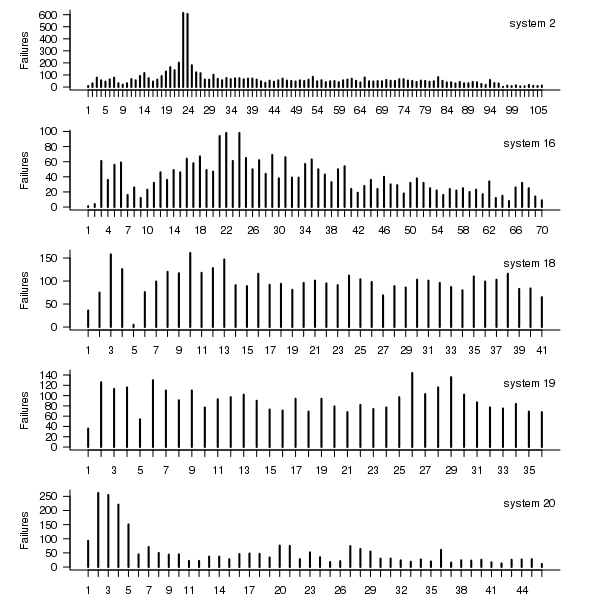
Figure 1. Total number of failures per 30-day interval for each LANL system.
Do some nodes failure more often than others?
The plot below shows the total number of failures for each node in the given system. Node 0 has many more failures than the other nodes (for node 0 of system 2 most of the failure data appears to be missing, so node 1 has the most failures). The distribution suggested by the analysis below is not changed if Node 0 is removed from the dataset.
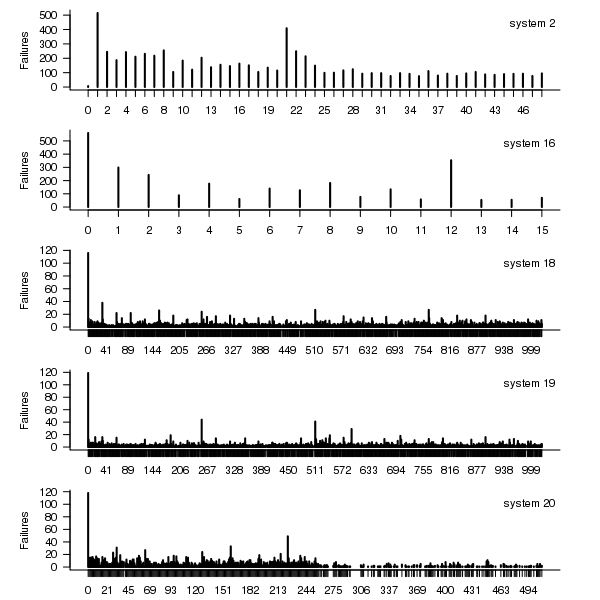
Figure 2. Total number of failures for each node in the given LANL system.
Fitting node uptimes
When plotted in units of 1 hour there is a lot of variability and so uptimes are binned into 10 hour units to help smooth the data. The number of uptimes in each 10-hour bin forms a discrete distribution and a [Cullen and Frey test] suggests that the negative binomial distribution might provide the best fit to the data; the Scroeder and Gibson analysis did not try the negative binomial distribution and of those they tried found the Weilbull distribution gave the best fit; the R functions were not able to fit this distribution to the data.
The plot below shows the 10-hour binned data fitted to a negative binomial distribution for systems 2 and 18. Visually the negative binomial distribution provides the better fit and the Akaiki Information Criterion values confirm this (see code for details and for the results on the other systems, which follow one of the two patterns seen in this plot).
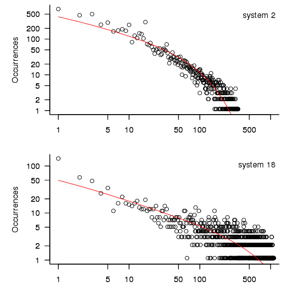
Figure 3. For systems 2 and 18, number of uptime intervals, binned into 10 hour interval, red line is fitted negative binomial distribution.
The negative binomial distribution is also the best fit for the uptime of the systems 16, 19 and 20.
The Poisson distribution often crops up in failure analysis. The quality of fit of a Poisson distribution to this dataset was an order of worse for all systems (as measured by AIC) than the negative binomial distribution.
Discussion
This analysis only compares how well commonly encountered distributions fit the data. The variability present in the datasets for all systems means that the quality of all fitted distributions will be poor and there is no theoretical justification for testing other, non-common, distributions. Given that the analysis is looking for the best fit from a chosen set of distributions no attempt was made to tune the fit (e.g., by forming a zero-truncated distribution).
Of the distributions fitted the negative binomial distribution has the lowest AIC and best fit visually.
As discussed in the section on [properties of distributions] the negative binomial distribution can be generated by a mixture of [Poisson distribution]s whose means have a [Gamma distribution]. Perhaps the many components in a node that can fail have a Poisson distribution and combined together the result is the negative binomial distribution seen in the uptime intervals.
The Weilbull distribution is often encountered with datasets involving some form of time between events but was not seen to be a good fit (for a continuous distribution) by a Cullen and Frey test and could not be fitted by the R functions used.
The characteristics of node uptime for two systems (i.e., 2 and 16) follows what might be thought of as a typical distribution of measurements, with some fattening in the tail, while two systems (i.e., 18 and 19) have very fat tails with indeed and system 20 sits between these two patterns. One system characteristic that matches this pattern is the number of nodes contained within it (with systems 2 and 16 having under 50, 18 and 19 having over 1,000 and 20 having around 500). The significantly difference in the size of the tails is reflected in the mean uptimes for the systems, given in the table above.
Summary of findings
The negative binomial distribution, of the commonly encountered distributions, gives the best fit to node uptime intervals for all systems.
There is over an order of magnitude variation in the mean uptime across some systems.
Recent Comments