Archive
Proposal for a change of approach to programming language teaching
In a previous post I explained why I think developers don’t really know any computer language, and in this post I want to outline how I think we should adapt to this reality and radically change the approach taken to teaching students about using a computer language. First, a couple of points:
- The programming community needs to change its attitude towards language knowledge from being an end in itself to being something that is ok to acquire on an as needed basis. Developers don’t need to know much about the programming language they use in order to get their job done, get over it. Spending time learning the ins and outs of a language’s semantics rarely provides a worthwhile return on investment compared to time spent learning something else, such as the application domain or customer requirements,
- designing a new, ‘simpler’ programming language is not a solution; the existing languages in common use are not going away anytime soon and creating a new general purpose language is only going to overload developers with more stuff to learn and yet another runtime system to interface to,
- we need to concentrate on suggestions about what students and developers should be doing and not what they should not be doing. This is not only a good teaching principle it avoids the problem of having to come up with a good list of things not to do (coding standard recommendations are very rarely based on any evidence apart from the proposers own point of view and even the ones that make it through peer review are little more than group think or a waste of time).
The response to the existing state of affairs should be to approach the teaching of programming languages as an exercise in teaching students only what they need to know to do useful work, rather than acting on the belief that students should strive to be experts in the language they use and burdening them with lots of pointless language details. The exact minimum-set of knowledge could vary across different industries and application domains, so the set might need to be a bit larger than the minimum to be on the safe side.
Invariably some developers will need to know more than the minimum-set, so we also need to figure out what ‘template’ knowledge (or whatever term is used, an alternative is behavior patterns or patterns of behavior) should be included in the next level of language knowledge, this can be documented and made available to anybody who wants to read it; there may or may not be more levels before a developer is told to go and read a reference book or the language reference manual to figure out what they need to know.
This is minimum-set approach, with the opportunity to progress to successively more detailed levels, is often used for learning human languages, computer languages are not any different.
I would expect there to be some variation in the minimum-set between different languages, and would resist the temptation to try and create a ‘common minimum’ until some experience had been gained in teaching single languages.
How would the minimum-set of language knowledge be chosen? Simple. Students need to learn those construct they are likely to use most of the time, and that question can be answered by measuring a large amount of existing source code. Results from measurements that have been made typically show a small number of constructs are used a large percentage of the time. For instance, measurements of C source find that the 33.2% of for-loops have the form: for (assignment ; identifier < identifier ; identifier++), where identifier might be two or more different identifiers; allowing the central test to have the form identifier < expression takes the percentage to over 50%. I would expect the same pattern of usage to occur in source written in other languages but don't have any number to back up that assertion.
Perhaps the most important pattern of (developer) behavior is what its discoverer, Jorma Sajaniemi, calls the roles of variables (each variable is used to hold a particular kind of information, e.g., most wanted holder, stepper, container, etc).
One pattern of behavior that I am more or less completely in the dark about is class/package usage. There is the famous book on design patterns which the authors did a good job of promoting, but I have yet to see any empirical evidence showing the claimed benefits. The analysis of class/package behavioral usage is non-trivial, but it can be done.
Would I insist that developers only use constructs list in the suggested minimum-set (plus possible extras)? No. The purpose of this proposal is to help students and developers learn what they need to know to get a job done. Figuring out what language constructs, if any, should be avoided at all costs is a very tough problem which at the end of the day might not be worth solving.
A minimum-set knowledge of the language being used does not imply poor quality code. Most code is simple anyway, the complicated stuff invariably revolves around the algorithms that need to be used, and a skillful developer is one who uses straightforward language constructs to create easy to maintain code, not one who writes code that relies on detailed knowledge of some language feature.
I expect this proposal to adopt a minimum-set approach to language teaching will draw an angry reaction from the cottage industry that makes its living from writing and giving seminars on the latest trends in language-X. Don't panic guys, managers are well aware that this kind of knowledge rarely has any impact of developer performance and the actual motivation for sending employees on such seminars is to keep them happy (it can be a much more effective way of keeping staff than simply giving them a pay rise).
Most developers don’t really know any computer language
What does it mean to know a language? I can count to ten in half a dozen human languages, say please and thank you, tell people I’m English and a few other phrases that will probably help me get by; I don’t think anybody would claim that I knew any of these languages.
It is my experience that most developers’ knowledge of the programming languages they use is essentially template based; they know how to write a basic instances of the various language constructs such as loops, if-statements, assignments, etc and how to define identifiers to have a small handful of properties, and they know a bit about how to glue these together.
There are many developers who can skilfully weave together useful programs from the hodgepodge of coding knowledge they happen to know (proving that little programming knowledge is needed to write useful programs).
The purpose of this post is not to complain about developers’ lack of knowledge of the programming languages they use; I appreciate that time spent learning about the application domain often gives a better return on investment compared to learning more about a language. The purpose is to suggest that the programming language community (e.g., teachers and tool producers) acknowledge how languages are primarily used and go with the flow rather than maintaining the fiction that developers know anything much about the languages they use and that they should acquire this knowledge to expert level; students should be taught the commonly encountered templates, not the general language rules, developers should be encouraged to use just the common templates (this will also have the side effect of reducing the effort needed to follow other peoples code since the patterns of usage will be familiar to many).
I suspect that many readers will disagree with the statement in this post’s title, and I need to provide more evidence before proposing (in another post) how we might adapt to the reality to be found in development teams.
The only evidence I can offer is my own experience; not a very satisfactory situation; a possible measurement approach discussed below. So what is this experience based evidence (I only claim to ‘know’ the handful of language I have written compiler front ends for, with other languages my usage follows the template form just like everybody else)?
- discussions with developers: individuals and development groups invariably have their own terminology for programming language constructs (my use of terminology appearing in the language definition usually draws blank stares and I have to make a stab at guessing what the local terms mean and using them if I want to be listened to); asking about identifier scoping or type compatibility rules (assuming that either of the terms ‘scope’ or ‘type compatibility’ is understood) usually results in a vague description of specific instances (invariably the commonly encountered situations),
- books that claim to teach a language often provide superficial coverage of the language semantics and concentrate on usage examples (because that is what is useful to their readers). Those books claiming to give insight into the depths of a language often contains many mistakes; perhaps the most well known example is Herbert Schildt’s “The Annotated ANSI C Standard”, Clive Feather’s review of the 1995 edition and Peter Seebach’s review of later versions,
- the word ‘Advanced’ has to appear in programming courses for professional developers with 3–10 years of experience because potential customers think they have reached an advanced level. In practice, such courses teach the basics and get away with it because most of the attendees don’t know them. My own experiences of teaching such courses is that outside of the walking people through the slides, the real teaching is about trying to undo some of the bad habits and misconceptions individuals have picked up over the years.
Recent graduate think they are an expert in the language used on their course because they probably have not met anybody who knows a lot more; some professional developers think they are language experts because the have lots of years of experience, in practice they tend to have spent those years essentially using what they originally learned and are now very adept with that small subset.
How might we measure the program language knowledge of the general developer population?
Software development question/answer sites such as Stack Overflow contain a wealth of information. I think I could write a function that did a reasonably good job of deducing the programming language, if any, being used in the question. Given the language definition (in some cases this might not exist, e.g., Perl and PHP) and the answers to the question of how do I figure out the language expertise of the person who wrote the answer?
First, we need to filter out those questions that are application related, with code being incidental. Latent Semantic Indexing could be used to locate the strongest connections between parts of the language specification and the non-source code answer text. If strong connections are found, the question would be assumed to be programming language related.
Developers only need surface knowledge to sprinkle any answer with phrases related to the language referred to; more in depth analysis is needed.
One idea is to process any code in the question/answer with a compiler capable of generating references to those parts of the language definition used during its semantic processing (ideally ‘part’ would be the sentence level, but I would settle for paragraph level or perhaps couple of paragraph level). A non-trivial overlap between the ‘parts’ references returned by the two searches would be a good indicator of programming language question. The big problem with this idea is complete lack of compilers supporting this language reference functionality (somebody please prove me wrong).
I am currently stumped for a practical technique for a non-superficial way of measuring developer language expertise. The 2013 Mining Software Repositories challenge is based on a dump of the questions/answers from Stack Overflow, I’m looking forward to seeing what useful information researchers extract from it.
Superoptimizers are back in vogue
There has always been the need for a few developers with in-depth knowledge of a particular cpu architecture to sit down and think very hard about how best to implement a snippet of code performing some operation in assembly language, e.g., library implementors wanting the tightest code for a critical inner loop or compiler writers who need to map from intermediate code to machine code.
In 1987 Massalin published his now famous paper that introduced the term Superoptimizer; a program that enumerates all possible combinations of instruction sequences until the shortest/fastest one producing the desired output from the given input is found (various heuristics were used to prune the search space e.g., only considering 15 or so opcodes, and the longest sequence it ever generated contained 12 instructions).
While the idea was widely talked about, it never caught on in practice (a special purpose branch eliminator was produced for GCC; Hacker’s Delight also includes a stand-alone system). Perhaps the guild of mindbogglingly-obtuse-but-fast-instruction-sequences black-balled it (apprentices have to spend several years doing nothing but writing assembly code for their chosen architecture, thinking about how to make it go faster and/or be shorter and only talk to other apprentices/members and communicate with non-converts exclusively about their latest neat sequence), or perhaps it was just a case of not invented here (writing machine code used to be something that even run-of-the-mill developers got to do every now and again), or perhaps it was not considered cost-effective to build a superoptimizer for a given project (I don’t know of anyone offering a generic tool that could be tailored for specific cases) or perhaps developers were happy to just ride the wave of continually faster processors.
It was not until 2008 with Bansal’s thesis that superoptimizer research started to take off (as in paper publication rate increased from once every five years to more than one a year). Bansal found a new market, binary translation i.e., translating the binary of a program built to run on one kind of cpu to run on a different kind of cpu, for instance the Mac 68K emulator.
Bansal and other researchers’ work was oriented towards relatively short instruction sequences. To be really useful, some way of handling longer sequences was needed.
A few days ago Stochastic Superoptimization arrived on the scene (or rather a paper describing it became available for download). Schkufza, Sharma and Aiken use Markov chain Monte Carlo methods to sample the possible instruction sequences rather than generating all of them. The paper gives a 116 instruction example from which the author’s tool removed 16 lines to produce code that went 1.6 times faster (only 30 ‘core’ instructions were given in paper); what is also very interesting is that the tool operates on compiler generated output (gcc/llvm), suggesting the usage build program, profile it and then stochastic superoptimize the hot spots.
Markov chains and Monte Carlo methods are trendy topics that researchers like to write about, so we will certainly see more papers in this area.
These days few developers have had hands-on experience with machine code, so the depth of expertise that was once easy to find is now rare, processors have many more weird and wonderful instructions often interacting with older instructions in obscure ways, and the cpu architecture landscape continues to change regularly. The time may have arrived for superoptimizers to be widely used by industry.
Of course, superoptimizers can work at any level of abstraction, including expression trees built directly from some complicated floating-point calculation that needs to be optimized for accuracy or speed.
Why is Cobol still popular in Japan?
Rummaging around the web for empirical software engineering data, I found a survey of programming language usage in Japan. This survey (based on 505 projects in 24 companies) has Cobol in the number two slot for 2012, a bit higher than I would have expected (it very rarely appears at all in US/UK ‘popularity’ lists):
Language       Projects
Java             822  28.2%
COBOL            464  15.9%
VB               371  12.7%
C                326  11.2%
Other languages  208   7.1%
C++              189   6.5%
Visual Basic.NET 136   4.7%
Visual C++       105   3.6%
C#               101   3.5%
PL/SQL            57   2.0%
Pro*C             23   0.8%
Excel(VBA)        18   0.6%
Developer2000     17   0.6%
ABAP              15   0.5%
HTML              14   0.5%
Delphi            11   0.4%
PL/I              10   0.3%
Perl              10   0.3%
PowerBuilder       7   0.2%
Shell              7   0.2%
XML                6   0.2%
A quick overview of Cobol for those readers who have never encountered it.
Cobol is a domain specific language ideally suited for business data processing in the 1960/70/80/90s. During this period computer memory was often measured in kilobytes, data came in an unbelievably wide range of different formats, operations on data mostly involved sorting and basic arithmetic, and output data format was/is very important. By “unbelievably wide range” think of lots of point-of-sale vendors deciding how their devices would write data to punch cards/paper tape/magnetic tape, just handling the different encodings that have been used for the plus/minus sign can make the head spin; combine the requirement that programs handle different data formats with tiny computer memory capacity, and you get data structure overlays that make C programmers look like rank amateurs, all the real action in Cobol programs occurs in the DATA DIVISION.
So where are we today? Companies use computers to solve a wider range of problems don’t they (so even if Cobol usage stayed the same its percentage usage should be low)? If point-of-sale terminals still produce a wide range of weird and wonderful data formats, isn’t it easy enough to write the appropriate libraries to convert (and we have much more storage these days)?
Why might Cobol still be so popular in Japan (and perhaps elsewhere, if anybody over 25 was included in the survey)? Some ideas:
- Cobol is still the best language to use for business data processing,
- the sample is not representative of the Japanese software development industry. As a government body perhaps the Information-Technology Promotion Agency primarily deals with large well established companies; the data came from a relatively small number of companies (i.e., 24),
- the Japanese are known for being conservative and maintaining traditions. Change is almost considered a necessity here in the West, this has led to the use of way too many programming languages in industry (I have previously written about what a mistake it is to invent a new language).
Sampling is now an issue in software engineering research
Data analysis in software engineering often has to make do with measurements extracted from the handful of measurable/measured instances at hand, but every now and again the abundance of stuff to measure is such that a subset has to be selected. How should the subset be selected?
Population sampling is a well established part of statistics, and a variety of terms have sprung up to label the various strategies used. I think ‘Accidental sampling’ accurately describes the provenance of many software engineering datasets seen in research papers and some of my work. It is quite common to see academic papers using exactly the same sample as previously published papers, perhaps a new term is needed to describe using samples that are identical to those used in previously papers: lazy sampling, coat-tail sampling…
Program source code, which was once so hard to obtain in any significant quantity, is now available by the terabyte load, a population that all but the fastest analysis and most general of questions warrant processing as a whole.
The question being asked can itself intrinsically lead to a reduction in the size of the population, e.g., properties of programs written in X, or programs with more than 10 active developers.
What should be the unit of sampling? The package making up a standalone system/library is a common choice (e.g., all the files in the tar or zip archive from which binaries are built); this can result in unexpected source files being included in the measurement process, such as test programs. A less common choice is to use individual source files as the sampling unit (it is so much easier to randomly select a list of packages, download, extract and measure them one by one).
Are the source file characteristics of the contents of 1,000 packages statistically very similar to 25,000 files obtained by randomly selecting 1 file from 25,000 packages? I don’t know.
A recent paper by Nagappan, Zimmermann and Bird proposes a sampling algorithm which looks like quota or coverage sampling in that candidate similarity to the current sample is used to decide whether to add that candidate (too much similarity results in exclusion). The authors misleadingly associate the term ‘representativeness’ with this algorithm, where common statistical usage of representative requires that if 40% of a population have attribute Z then 40% of a sample’s members will have this attribute (within sampling tolerances).
If software engineering research is to be useful to commercial software engineering, any discoveries need to be applicable to samples outside of those used in the original analysis. At the moment researchers are having a hard enough time finding any useful patterns in their data, this is not a reason to continue with the practice of coat-tail sampling and we all need to start addressing sampling issues.
Break even ratios for development investment decisions
Developers are constantly being told that it is worth making the effort when writing code to make it maintainable (whatever that might be). Looking at this effort as an investment what kind of return has to be achieved to make it worthwhile?
Short answer: The percentage saving during maintenance has to be twice as great as the percentage investment during development to break even, higher ratio to do better.
The longer answer is below as another draft section from my book Empirical software engineering with R book. As always comments and pointers to more data welcome. R code and data here.
Break even ratios for development investment decisions
Upfront investments are often made during software development with the aim of achieving benefits later (e.g., reduced cost or time). Examples of such investments include spending time planning, designing or commenting the code. The following analysis calculates the benefit that must be achieved by an investment for that investment to break even.
While the analysis uses years as the unit of time it is not unit specific and with suitable scaling months, weeks, hours, etc can be used. Also the unit of development is taken to be a complete software system, but could equally well be a subsystem or even a function written by one person.
Let  be the original development cost and
  the yearly maintenance costs, we start by keeping things simple and assume is the same for every year of maintenance; the total cost of the system over
  years is:

If we make an investment of  % in reducing future maintenance costs with the expectations of achieving a benefit of
  %, the total cost becomes:
 + y*m*(1+i)*(1-b)")
and for the investment to break even the following inequality must hold:
 + y*m*(1+i)*(1-b) < d + y*m")
expanding and simplifying we get:

or:

If the inequality is true the ratio  is the primary contributor to the right-hand-side and must be greater than 1.
A significant problem with the above analysis is that it does not take into account a major cost factor; many systems are replaced after a surprisingly short period of time. What relationship does the ratio need to have when system survival rate is taken into account?
Let  be the percentage of systems that survive each year, total system cost is now:

where *(1-b)")
Summing the power series for the maximum of years that any system in a company’s software portfolio survives gives:
}/{1 - s}")
and the break even inequality becomes:
} < {b}/{i} + b")
The development/maintenance ratio is now based on the yearly cost multiplied by a factor that depends on the system survival rate, not the total maintenance cost
If we take >= 5 and a survival rate of less than 60% the inequality simplifies to very close to:

telling us that if the yearly maintenance cost is equal to the development cost (a situation more akin to continuous development than maintenance and seen in 5% of systems in the IBM dataset below) then savings need to be at least twice as great as the investment for that investment to break even. Taking the mean of the IBM dataset and assuming maintenance costs spread equally over the 5 years, a break even investment requires savings to be six times greater than the investment (for a 60% survival rate).
The plot below gives the minimum required saving/investment ratio that must be achieved for various system survival rates (black 0.9, red 0.8, blue 0.7 and green 0.6) and development/yearly maintenance cost ratios; the line bundles are for system lifetimes of 5.5, 6, 6.5, 7 and 7.5 years (ordered top to bottom)
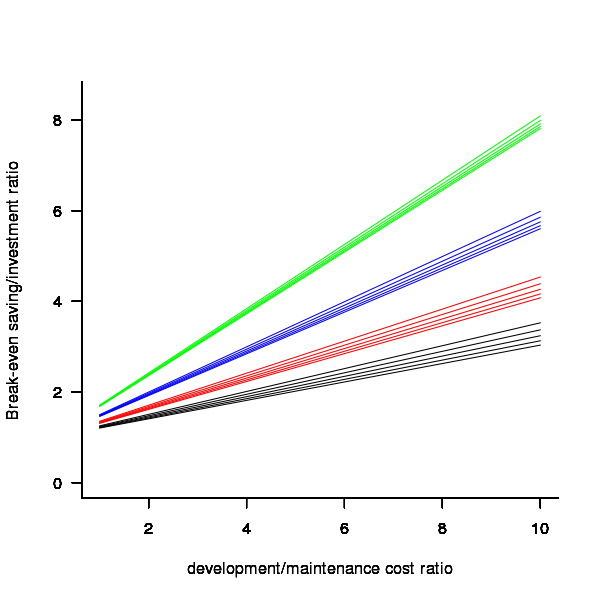
Figure 1. Break even saving/investment ratio for various system survival rates (black 0.9, red 0.8, blue 0.7 and green 0.6) and development/maintenance ratios; system lifetimes are 5.5, 6, 6.5, 7 and 7.5 years (ordered top to bottom)
Development and maintenance costs
Dunn’s PhD thesis <book Dunn_11> lists development and total maintenance costs (for the first five years) of 158 software systems from IBM. The systems varied in size from 34 to 44,070 man hours of development effort and from 21 to 78,121 man hours of maintenance.
The plot below shows the ratio of development to five year maintenance costs for the 158 software systems. The mean value is around one and if we assume equal spending during the maintenance period then  .
.
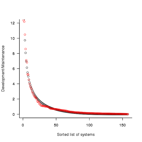
Figure 2. Ratio of development to five year maintenance costs for 158 IBM software systems sorted in size order. Data from Dunn <book Dunn_11>.
The best fitting common distribution for the maintenance/development ratio is the <Beta distribution>, a distribution often encountered in project planning.
Is there a correlation between development man hours and the maintenance/development ratio (e.g., do smaller systems tend to have a lower/higher ratio)? A Spearman rank correlation test between the maintenance/development ratio and development man hours gives:
|
showing very little connection between the two values.
Is the data believable?
While a single company dataset might be thought to be internally consistent in its measurement process, IBM is a very large company and it is possible that the measurement processes used were different.
The maintenance data applies to software systems that have not yet reached the end of their lifespan and is not broken down by year. Any estimate of total or yearly maintenance can only be based on assumptions or lifespan data from other studies.
System lifetime
A study by Tamai and Torimitsu <book Tamai_92> obtained data on the lifespan of 95 software systems. The plot below shows the number of systems surviving for at least a given number of years and a fit of an <Exponential distribution> to the data.
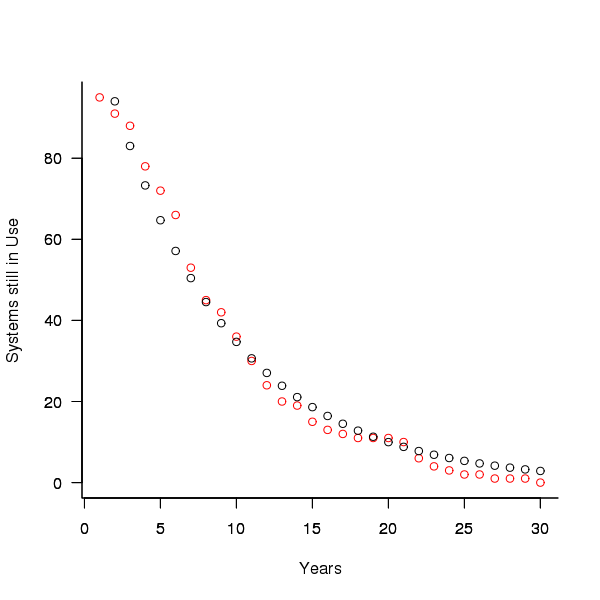
Figure 3. Number of software systems surviving to a given number of years (red) and an exponential fit (black, data from Tamai <book Tamai_92>).
The nls function gives  as the best fit, giving a half-life of 5.4 years (time for the number of systems to reduce by 50%), while rounding to
  gives a half-life of 6.6 years and reducing to
  a half life of 4.6 years.
It is worrying that such a small change to the estimated fit can have such a dramatic impact on estimated half-life, especially given the uncertainty in the applicability of the 20 year old data to today’s environment. However, the saving/investment ratio plot above shows that the final calculated value is not overly sensitive to number of years.
Is the data believable?
The data came from a questionnaire sent to the information systems division of corporations using mainframes in Japan during 1991.
It could be argued that things have stabilised over the last 20 years ago and complete software replacements are rare with most being updated over longer periods, or that growing customer demands is driving more frequent complete system replacement.
It could be argued that large companies have larger budgets than smaller companies and so have the ability to change more quickly, or that larger companies are intrinsically slower to change than smaller companies.
Given the age of the data and the application environment it came from a reasonably wide margin of uncertainty must be assigned to any usage patterns extracted.
Summary
Based on the available data an investment during development must recoup a benefit during maintenance that is at least twice as great in percentage terms to break even:
- systems with a yearly survival rate of less than 90% must have a benefit/investment rate greater than two if they are to break even,
- systems with a development/yearly maintenance rate of greater than 20% must have a benefit/investment rate greater than two if they are to break even.
The availanble software system replacement data is not reliable enough to suggest any more than that the estimated half-life might be between 4 and 8 years.
This analysis only considers systems that have been delivered and started to be used. Projects are cancelled before reaching this stage and including these in the analysis would increase the benefit/investment break even ratio.
Agreement between code readability ratings given by students
I have previously written about how we know nothing about code readability and questioned how the information content of expressions might be calculated. Buse and Weimer ran a very interesting experiment that asked subjects to rate short code snippets for readability (somebody please rerun this experiment using professional software developers).
I’m interested in measuring how well different students subjects agree with each other (I have briefly written about this before).
Short answer: Very little agreement between individual pairs, good agreement between rankings aggregated by year.
The longer answer is below as another draft section from my book Empirical software engineering with R book. As always comments welcome. R code and data here.
Readability
Source code is often said to have an attribute known as
A study by Buse and Weimer <book Buse_08> asked Computer Science students to rate short snippets of Java source code on a scale of 1 to 5. Buse and Weimer then searched for correlations between these ratings and various source code attributes they obtained by measuring the snippets.
Humans hold diverse opinions, have fragmented knowledge and beliefs about many topics and vary in their cognitive abilities. Any study involving human evaluation that uses an open ended problem on which subjects have had little experience is likely to see a wide range of responses.
Readability is a very nebulous term and students are unlikely to have had much experience working with source code. A wide range of responses is to be expected and the analysis performed here aims to check the degree of readability rating agreement between the subjects.
Data
The data made available by Buse and Weimer are the ratings, on a scale of 1 to 5, given by 121 students to 100 snippets of source code. The student subjects were drawn from those taking first, second and third/fourth year Computer Science degree courses and postgraduates at the researchers’ University (17, 65, 31 and 8 subjects respectively).
The postgraduate data was not used in this analysis because of the small number of subjects.
The source of the code snippets is also available but not used in this analysis.
Is the data believable?
The subjects were not given any instructions on how to rate the code snippets for readability. Also we don’t know what outcome they were trying to achieve when rating, e.g., where they rating on the basis of how readable they personally found the snippets to be, or rating on the basis of the answer they would expect to give if they were being tested in an exam.
The subjects were students who are learning about software development and many of them are unlikely to have had any significant development experience outside of the teaching environment. Experience shows that students vary significantly in their ability to read and write source code and a non-trivial percentage do not go on to become software developers.
Because the subjects are at an early stage of learning about code it is to be expected that their opinions about readability will change while they are rating the 100 snippets. The study did not include multiple copies of some snippets, this would have enabled the consistency of individual subject responses to be estimated.
The results of many studies <book Annett_02> has shown that most subject ratings are based on an ordinal scale (i.e., there is no fixed relationship between the difference between a rating of 2 and 3 and a rating of 3 and 4), that some subjects are be overly generous or miserly in their rating and that without strict rating guidelines different subjects apply different criteria when making their judgements (which can result a subject providing a list of ratings that is inconsistent with every other subject).
Readability is one of those terms that developers use without having much idea what they and others are really referring to. The data from this study can at most be regarded as treating readability to be whatever each subject judges it to be.
Predictions made in advance
Is the readability rating given to code snippets consistent between different students on a computer science course?
The hypothesis is that the between student consistency of the readability rating given to code snippets improves as students progress through the years of attending computer science courses.
Applicable techniques
There are a variety of techniques for estimating rater agreement. <Krippendorff’s alpha> can be applied to ordinal ratings given by two or more raters and is used here.
Subjects do not have to give the same rating to share some degree of consistent response. Two subjects may share a similar pattern of increasing/decreasing/stay the same ratings across snippets. The <Spearman rank correlation> coefficient can be used to measure the correlation between the rank (i.e., relative value within sequence) of two sequences.
Results
When creating the snippets the researchers had no method of estimating what rating subjects would give to them and so there is no reason to expect a uniform distribution of rating values or any other kind of distribution of rating values.
The figure below is a boxplot of the rating of the first 50 code snippets rated by second year students and suggests that many subject ratings are within ±1 of each other.
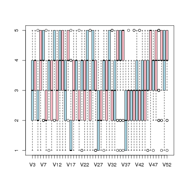
Figure 1. Boxplot of ratings given to snippets 1 to 50 by second year students (colors used to help distinguish boxplots for each snippet).
Between subject rating agreement
The Krippendorff alpha and mean Spearman rank correlation coefficient (the coefficient is calculated for every pair of subjects and the mean value taken) was obtained using the kripp.alpha and meanrho functions from the irr package (a <Jackknife> was used to obtain the following 95% confidence bounds):
Krippendorff's alpha cs1: 0.1225897 0.1483692 cs2: 0.2768906 0.2865904 cs4: 0.3245399 0.3405599 mean Spearman's rho cs1: 0.1844359 0.2167592 cs2: 0.3305273 0.3406769 cs4: 0.3651752 0.3813630 |
Taken as a whole there is a little of agreement. Perhaps there is greater consensus on the readability rating for a subset of the snippets. Recalculating using only using those snippets whose rated readability across all subjects, by year, has a standard deviation less than 1 (around 22, 51 and 62% of snippets respectively) shows some improvement in agreement:
Krippendorff's alpha cs1: 0.2139179 0.2493418 cs2: 0.3706919 0.3826060 cs4: 0.4386240 0.4542783 mean Spearman's rho cs1: 0.3033275 0.3485862 cs2: 0.4312944 0.4443740 cs4: 0.4868830 0.5034737 |
Between years comparison of ratings
The ratings from individual subjects is only available for one of their years at University. Aggregating the answers from all subjects in each year is one method of obtaining readability information that can be used to compare the opinions of students in different years.
How can subject ratings be aggregated to rank the 100 code snippets in order of what a combined group consider to be readability? The relatively large variation in mean value of the snippet ratings across subjects would result in wide confidence bounds for an aggregate based on ratings. Mapping each subject’s rating to a ranking removes the uncertainty caused by differences in mean subject ratings.
With 100 snippets assigned a rating between 1 and 5 by each subject there are going to be a lot of tied rankings. If, say, a subject gave 10 snippets a rating of 5 the procedure used is to assign them all the rank that is the mean of the ranks the 10 of them would have occupied if their ratings had been very slightly different, i.e., (1+2+3+4+5+6+7+8+9+10)/10 = 5.5. This process maps each students readability ratings to readability rankings, the next step is to aggregate these individual rankings.
The R_package[RankAggreg] package contains a variety of functions for aggregating a collection rankings to obtain a group ranking. However, these functions use the relative order of items in a vector to denote rank, and this form of data representations prevents them supporting ranked lists containing items having the same rank.
For this analysis a simple aggregate ranking algorithm using Borda’s method <book lin_10> was implemented. Borda’s method for creating an aggregate ranking operates on one item at a time, combining all of the subject ranks for that item into a single rank. Methods for combining ranks include taking their mean, their geometric mean and the square-root of the sum of their squares; the mean value was used for this analysis.
An aggregate ranking was created for subjects in years one, two and four and the plot below compares the ranking between 1st/2nd year students (left) and 2nd/4th year students (right). The order of the second year student snippet rankings have been sorted and the other year rankings for the snippets mapped to the corresponding position.
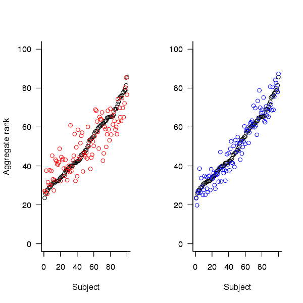
Figure 2. Aggregated ranking of snippets by subjects in years 1 and 2 (red and black) and years 2 and 4 (black and blue). Snippets have been sorted by year 2 ranking.
The above plot seems to show that at the aggregated year level there is much greater agreement between the 2nd/4th years than any other year pairing and measuring the correlation between each of the years using <Kendall’s tau>:
cs1.tau cs2.tau cs3.tau 0.6627602 0.6337914 0.8199636 |
confirms the greater agreement between this aggregate year pair.
Individual subject correlation to year aggregate ranking
To what extend to subject ratings correlate with their corresponding year aggregate? The following plot gives the correlation, using Kendall’s tau, between each subject and their corresponding year aggregate ranking.
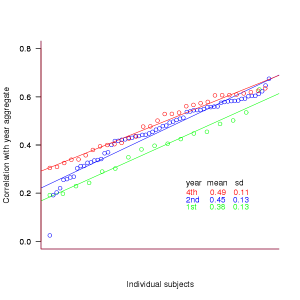
Figure 3. Correlation, using Kendall’s tau, between each subject and their corresponding year aggregate ranking.
The least squares fit shows that the variation in correlation across subjects in any year is very similar (removal of outliers in year 2 would make the lines almost parallel); the mean again shows a correlation that increases with year.
Discussion
The extent to which this study’s calculated values of rater agreement and correlation are considered worthy of further attention depends on the use to which the results will be put.
- From the perspective of trained raters the subject agreement in this study is very low and the rating have no further use.
- From the research perspective the results show that the concept of readability in the computer science student population has some non-zero substance to it that might be worth further study.
- From an overall perspective this study provides empirical evidence for a general lack of consensus on what constitutes readability.
It is not surprising that there is little agreement between student subjects on their readability rating, they are unlikely to have had much experience reading code and have not had any training in rating code for readability.
Professional developers will have spent years working with code and this experience is likely to have resulted in the creation of stable opinions on code readability. While developers usually work with code that is much longer than the few lines contained in the snippets used by Buse and Weimer, this experiment format is easy to administer and supports a fine level of control, i.e., allows a small set of source attributes of interest to be presented while excluding those not of interest. Repeating this study using such people as subjects would show whether this experience results in convergence to general agreement on the readability rating of code.
Summary of findings
The agreement between students readability ratings, for short snippets of code, improves as the students progress through course years 1 to 4 of a computer science degree.
While there is very good aggregated group agreement on the relative ranking of the readability of code snippets there is very little agreement between pairs of individuals.
- Two students chosen at random from within a year will have a low Spearman rank correlation coefficient for their rating of code snippet readability.
- Taken as a yearly aggregate there is a high degree of agreement between years two and four and less, but still good agreement between year 1 and other years.
- There is a broad range of correlations, from poor to good, between year aggregates and student subjects in the corresponding year.
Sequence generation with no duplicate pairs
Given a fixed set of items (say, 6 A, 12 B and 12 C) what algorithm will generate a randomised sequence containing all of these items with any adjacent pairs being different, e.g., no AA, BB or CC in the sequence? The answer would seem to be provided in my last post. However, turning this bit of theory into practice uncovered a few problems.
Before analyzing the transition matrix approach let’s look at some of the simpler methods that people might use. The most obvious method that springs to mind is to calculate the expected percentage of each item and randomly draw unused items based on these individual item percentages, if the drawn item matches the current end of sequence it is returned to the pool and another random draw is made. The following is an implementation in R:
seq_gen_rand_total=function(item_count) { last_item=0 rand_seq=NULL # Calculate each item's probability item_total=sum(item_count) item_prob=cumsum(item_count)/item_total while (sum(item_count) > 0) { # To recalculate on each iteration move the above two lines here. r_n=runif(1, 0, 1) new_item=which(r_n < item_prob)[1] # select an item if (new_item != last_item) # different from last item? { if (item_count[new_item] > 0) # are there any of these items left? { rand_seq=c(rand_seq, new_item) last_item=new_item item_count[new_item]=item_count[new_item]-1 } } else # Have we reached a state where a duplicate will always be generated? if ((length(which(item_count != 0)) == 1) & (which(item_count != 0)[1] == last_item)) return(0) } return(rand_seq) } |
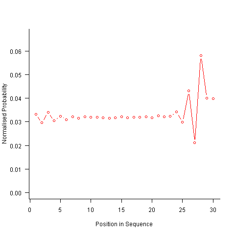
For instance, with 6 A, 12 B and 12 C, the expected probability is 0.2 for A, 0.4 for B and 0.4 for C. In practice if the last item drawn was a C then only an A or B can be selected and the effective probability of A is effectively increased to 0.3333. The red circles in the figure below show the normalised probability of an A appearing at different positions in the sequence of 30 items (averaged over 200,000 random sequences); ideally the normalised probability is 0.0333 for all positions in the sequence In practice the first position has the expected probability (there is no prior item to disturb the probability), the probability then jumps to a higher value and stays sort-of the same until the above-average usage cannot be sustained any more and there is a rapid decline (the sudden peak at position 29 is an end-of-sequence effect I talk about below).
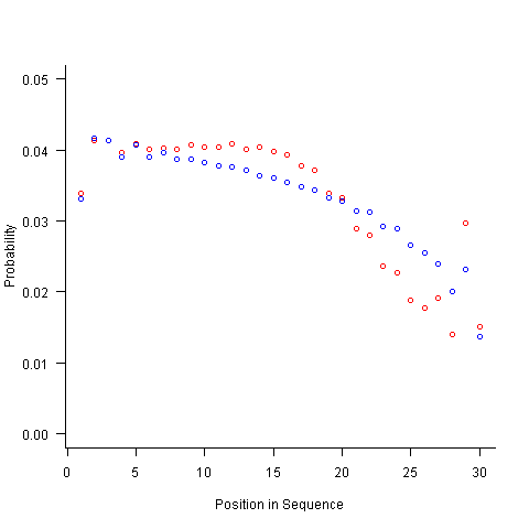
What might be done to get closer to the ideal behavior? A moments thought leads to the understanding that item probabilities change as the sequence is generated; perhaps recalculating item probabilities after each item is generated will improve things. In practice (see blue dots above) the first few items in the sequence have the same probabilities (the slight differences are due to the standard error in the samples) and then there is a sort-of consistent gradual decline driven by the initial above average usage (and some end-of-sequence effects again).
Any sequential generation approach based on random selection runs the risk of reaching a state where a duplicate has to be generated because only one kind of item remains unused (around 80% and 40% respectively for the above algorithms). If the transition matrix is calculated on every iteration it is possible to detect the case when a given item must be generated to prevent being left with unusable items later on. The case that needs to be checked for is when the percentage of one item is greater than 50% of the total available items, when this occurs that item must be generated next, e.g., given (1 A, 1 B, 3 C) a C must be generated if the final list is to have the no-pair property.
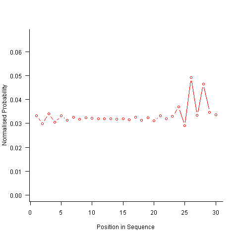
Now the transition matrix approach. Here the last item generated selects the matrix row and a randomly generated value selects the item within the row. Let’s start by generating the matrix once and always using it to select the next item; the resulting normalised probability stays constant for much longer because the probabilities in the transition matrix are not so high that items get used up early in the sequence. There is a small decline near the end and the end-of-sequence effects kick in sooner. Around 55% of generated sequences failed because two of the items were used up early leaving a sequence of duplicates of the remaining item at the end.
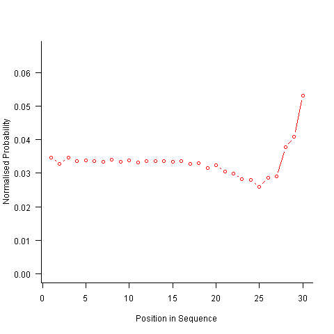
Finally, or so I thought, the sought after algorithm using a transition matrix that is recalculated after every item is generated. Where did that oscillation towards the end of the sequence come from?
After a some head scratching I realised that the French & Perruchet algorithm is based on redistribution of the expected number of items pairs. Towards the end of the sequence there is a growing probability that the number of remaining As will have dropped to one; it is not possible to create an AA pair from only one A and the assumptions behind the transition matrix calculation break down. A good example of the consequences of this breakdown is the probability distribution for the five item sequences that the algorithm might generate from (1 A, 2 B, 2 C); an A will never appear in position 2 of the sequence:
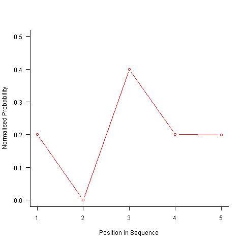
After various false starts I decided to update the French & Perruchet algorithm to include and end-of-sequence state. This enabled me to adjust the average normalised probability of the main sequence (it has be just right to avoid excess/missing probability inflections at the end), but it did not help much with the oscillations in the last five items (it has to be said that my updated calculations involve a few hand-waving approximations of their own).
I found that a simple, ad hoc solution to damp down the oscillations is to increase any single item counts to somewhere around 1.3 to 1.4. More thought is needed here.
Are there other ways of generating sequences with the desired properties? French & Perruchet give one in their paper; this generates a random sequence, removes one item from any repeating pairs and then uses a random insert and shuffle algorithm to add back the removed items. Robert French responded very promptly to my queries about end-of-sequence effects, sending me a Matlab program implementing an updated version of the algorithm described in the original paper that he tells does not have this problem.
The advantage of the transition matrix approach is that the next item in the sequence can be generated on an as needed basis (provided the matrix is calculated on every iteration it is guaranteed to return a valid sequence if one exists; of course this recalculation removes some randomness for the sequence because what has gone before has some influence of the item distribution that follows). R code used for the above analysis.
I have not been able to locate any articles describing algorithms for generating sequences that are duplicate pair free and would be very interested to hear of any reader experiences.
Transition probabilities when adjacent sequence items must be different
Generating a random sequence from a fixed set of items is a common requirement, e.g., given the items A, B and C we might generate the sequence BACABCCBABC. Often the randomness is tempered by requirements such as each item having each item appear a given number of times in a sequence of a given length, e.g., in a random sequence of 100 items A appears 20 times, B 40 times and C 40 times. If there are rules about what pairs of items may appear in the sequence (e.g., no identical items adjacent to each other), then sequence generation starts to get a bit complicated.
Let’s say we want our sequence to contain: A 6 times, B 12 times and C 12 times, and no same item pairs to appear (i.e., no AA, BB or CC). The obvious solution is to use a transition matrix containing the probability of generating the next item to be added to the end of the sequence based on knowing the item currently at the end of the sequence.
My thinking goes as follows:
- given A was last generated there is an equal probability of it being followed by B or C,
- given B was last generated there is a 6/(6+12) probability of it being followed by A and a 12/(6+12) probability of it being followed by C,
- given C was last generated there is a 6/(6+12) probability of it being followed by A and a 12/(6+12) probability of it being followed by B.
giving the following transition matrix (this row by row approach having the obvious generalization to more items):
                 Second item
               A      B       C
          A    0     .5      .5
First
item      B   .33     0      .67

C .33 .67 0 |
Having read Generating constrained randomized sequences: Item frequency matters by Robert M. French and Pierre Perruchet (from whom I take these examples and algorithm on which the R code is based), I now know this algorithm for generating transition matrices is wrong. Before reading any further you might like to try and figure out why.
The key insight is that the number of XY pairs (reading the sequence left to right) must equal the number of YX pairs (reading right to left) where X and Y are different items from the fixed set (and sequence edge effects are ignored).
If we take the above matrix and multiply it by the number of each item we get the following (if A occurs 6 times it will be followed by B 3 times and C 3 times, if B occurs 12 times it will be followed by A 4 times and C 8 times, etc):
                 Second item
               A      B       C
          A    0      3       3
First
item      B    4      0       8

C 4 8 0 |
which implies the sequence will contain AB 3 times when counted forward and BA 4 times when counted backwards (and similarly for AC/CA). This cannot happen, the matrix is not internally consistent.
The correct numbers are:
                 Second item
               A      B       C
          A    0      3       3
First
item      B    3      0       9

C 3 9 0 |
giving the probability transition matrix:
                 Second item
               A      B       C
          A    0     .5      .5
First
item      B   .25     0      .75

C .25 .75 0 |
This kind of sequence generation occurs in testing and I wonder how many people have made the same mistake as me and scratched their heads over small deviations from the expected results.
The R code to calculate the transition matrix is straight forward but obscure unless you have the article to hand:
# Calculate expression (3) from: # Generating constrained randomized sequences: Item frequency matters # Robert M. French and Pierre Perruchet transition_count=function(item_count) { N_total=sum(item_count) # expected number of transitions ni_nj=(item_count %*% t(item_count))/(N_total-1) diag(ni_nj) = 0 # expected number of repeats d_k=item_count*(item_count-1)/(N_total-1) # Now juggle stuff around to put the repeats someplace else n=sum(ni_nj) n_k=rowSums(ni_nj) s_k=n - 2*n_k R_i=d_k / s_k R=sum(R_i) new_ij=ni_nj*(1-R) + (n_k %*% t(R_i)) + (R_i %*% t(n_k)) diag(new_ij)=0 return(new_ij) } transition_prob=function(item_count) { tc=transition_count(item_count) tp=tc / rowSums(tc) # relies on recycling return(tp) } |
the following calls:
transition_count(c(6, 12, 12)) transition_prob(c(6, 12, 12)) |
return the expected results.
French and Perruchet provide an Excel spreadsheet (note this contains a bug, the formula in cell F20 should start with F5 rather than F6).
Impact of compiler optimization level on recovery from a hardware error
I have previously written about cosmic-ray induced faults in cpus and some of the compiler research being done to recover from such hardware faults. If your program is executing in an environment where radiation may cause hardware bit-flips to occur and you don’t have access to a research compiler providing some level of recovery, is it better to compile with high or low levels of optimization?
Short answer: Using gcc with optimization options O2 or O3 reduces the probability that a bit-flip will change the external behavior of a program, compared to option O0.
The longer answer is below as another draft section from my book Empirical software engineering with R book. As always comments welcome.
Software masking of hardware faults
Like all hardware cpus are subject to intermittent faults, these faults may flip the value of a bit in a program visible register, a bit in an executable instruction or some internal processor state (causes include cosmic rays, and electrical wear of the material from which circuits are built).
If a bit-flip randomly occurs at some point during a program’s execution, is it less likely to effect external program behavior when the code has been built with high levels of compiler optimization or built with optimization disabled or at a low level?
- many optimizations reduce the number of instructions executed (reducing execution time reduces the probability of encountering a bit-flip) and makes more efficient use of registers (e.g., keeping needed values in registers over longer periods of time and reducing the time intervals when a registers is not in use; which increases the probability that a bit-flip will propagate to external behavior),
- fewer compiler optimizations is likely to result in an increased number of instructions executed (increasing the probability that a bit-flip will occur during program execution) and results in lower register usage efficiency (e.g., longer periods of time between the last use of register contents and a new value being loaded; increasing the probability that a bit-flip will modify a value that is never used again).
A study by Cook and Zilles flipped one bit in an executing program (100 evenly distributed points in the program were chosen and 100 instructions from each of those points were used as fault injection points, giving a total of 10,000 individual tests to be run) and monitored the impact on subsequent execution; this process was repeated between 32 and 244 times for each injection point, once for every bit in the 32-bit instruction, zero, one or two of its 64-bit input registers and one possible 64-bit output result register (i.e., the bit-flip only involved the current instruction and its input/output, not the contents of any other register or main memory).
The monitoring process consisted of two parallel executions containing the modified processor state and the unmodified processor state. The behavior of the two executions were compared to see if the fault did not propagate (a passing trial, e.g., a bit-wise AND of a register with 0xff when a bit-flip has been applied to one of the top 24 bits of the register, also the values in a branch not-equal are usually not-equal and a bit-flip is likely to maintain that state), caused a failure (either due to a compulsory event caused by a hardware trap such as an invalid instruction or an incorrectly aligned memory access, or what was called an error model event such as a control flow mismatch or writing a different value to storage), or is inconclusive (pass/fail did not occur within 10,000 executed instructions of the fault injection point).
Data
The available data consists of the normalised number of program executions having one of the behaviors pass, fail (compulsory), fail (error model, broken down into control flow and store related cases) or inconclusive for nine programs from the SPEC2000 integer benchmark compiled using gcc version 4.0.2 and the DEC C compiler (henceforth called O0, O2 and O3, for osf the O4 option was used.
There are nine measurements for each of the nine SPEC programs, repeated at 3 optimization levels for gcc and once for osf (the osf data is not analysed here).
Is the data believable?
Injecting bit-flip faults at all points in a program and monitoring for subsequence changes in external behavior would be an enormous task, sets of 100 instructions starting from 100 locations appears to be an unbiased sample.
The error model used checks for changes of control flow and different values being stored to memory, it does not check for actual changes in external program behavior. This model biases the measurements in favour of more bit-flips being counted as generating an error than would occur in practice.
Predictions made in advance
Does compiler optimization level change the probability that a bit-flip will cause a change in external program behavior?
No hypothesis is proposed suggesting that compiler optimization level will increase, decrease or have no effect on the probability of a bit-flip effecting external program behavior.
Applicable techniques
The data was originally a count of the number of instances and this has been normalised to a value between 0 and 100. The same number of programs were executed at all optimization levels.
Non-parametric techniques have to be used because nothing is known about the distribution of values.
The [Wilcoxon signed-rank test] is a test for two dependent samples while the [Mann-Whitney U test] is a test for two independent samples. To what extent does running gcc at different optimization levels make it a different compiler? Given that we are testing for the possibility that compiler optimizations do effect the results then it is necessary to treat the samples as being independent.
The function wilcox.test will perform a Mann-Whitney test if the parameter paired is FALSE (the default) and will generate a confidence interval if the parameter conf.int is TRUE (the default is FALSE).
Results
The Mann-Whitney test of the various measurements obtained using the O2 and O3 options finds no worthwhile difference between them. There are interesting differences in the values obtained using both of two options and the O0 option, as follows:
- Pass
-
Comparing percentage of pass behaviors for
O0andO2we see: p-values = 0.005 and 0.005
> wilcox.test(gcc.o0$pass.masked, gcc.o2$pass.masked, conf.int=TRUE)
        Wilcoxon rank sum test with continuity correction

data:  gcc.o0$pass.masked and gcc.o2$pass.masked
W = 8, p-value = 0.004697
alternative hypothesis: true location shift is not equal to 0
95 percent confidence interval:
 -15.449995  -2.020001
sample estimates:
difference in location
             -7.480088
The wilcox.test function returns an estimate of the difference between the two means and a negative value occurs if the second argument (the higher optimization level in this case) has a greater mean than the first argument (which is always the O0 option in these results).
O0/O3 95% confidence interval: -15.579959 -1.909965, mean: -4.780058
- Fail (compulsory)
-
-
Memory protection fault: pvalues = 0.002 and 0.005
O0/O295%: 2.1 7.5, mean: 4.9
O0/O395%: 1.9 7.3, mean: 4.1 -
Invalid instruction: p-values = 0.045 and 0.053
O0/O295%: -8.0e-01 -4.9e-08, mean: -0.5
O0/O395%: -6.4e-01 5.1e-06, mean: -0.3
-
Memory protection fault: pvalues = 0.002 and 0.005
- Fail (error model)
-
-
Control flow: p-values = 0.0008 and 0.002
O0/O295%: -10.8 -3.8, mean: -7.0
O0/O395%: -10.5 -3.7, mean: -6.8 -
Store related: p-values = 0.002 and 0.003
O0/O295%: 4.78 22.02, mean: 11.24
O0/O395%: 4.93 18.78, mean: 10.51
-
Control flow: p-values = 0.0008 and 0.002
Discussion
O2 and O3 options differences
The issue of optimization performance differences between the gcc O2 and O3 options is covered in [another section] of this book. That analysis found that the only difference between the two options was an increase in code size with O3, probably because of function inlining.
If there is no significant difference in the code generated by the O2/O3 options then no difference in bit-flip behavior is expected, and none was seen.
Changes in failure rates
The results show a decrease in store related errors at high optimization levels and an increase in control flow related errors. Why is this?
Optimizing register usage is a very important optimization and one of its consequences is a reduction in the number of stores to memory and loads having a corrupted address triggering a protection fault . A reduction in the number of memory related instructions executed will feed through into a reduction in the number of failures classified as store related or memory protection faults and this is seen in the shift in mean value of fails between high and low optimization levels.
Keeping a value containing an injected bit-flip in a register for a longer period of program execution (rather than being stored to memory and loaded back later) provides the opportunity for it to work its way through subsequent instructions and either disappear (being counted as a pass) or cause a control flow failure. It is likely that some of the change stored values flagged by the error model do not an impact on external program behavior and the pass count at low optimization levels is lower than would occur in practice.
Changes in pass rate
The additional optimizations of register usage enabled by the O2/O3 options reduces memory accesses which leads to a reduction in memory protection errors, an unrecoverable fault under all circumstances. The numbers suggest that while this is a major factor in the increased pass rate, contributions are made by other sources, e.g., bit-flips not contributing to the result calculated by an instruction; the data is not sufficiently detailed to enable a reliable estimate of this contribution to be made.
The pass rate is likely to be an underestimate because the error model classifies storing a different value as a failure, however the different value might not result in a change of external program behavior, e.g., the value stored might never be used again. Some of the stores classified as errors for the O0 option have no lasting affect in practice (and being kept in registers for O2/O3 had the opportunity to be masked out). No data is available for enable an estimate to be made for the percentage of these bit-flips have no lasting affect.
The average pass rate for gcc using the O0 option was 28% and this increased to around 36% when the O2/O3 options were used.
Other processors
How likely is it that the bit-flip pass rates seen on the Alpha (average of 36% for high optimization, 28% for low) would also occur on other processors?
The Alpha registers contain 64-bit and instructions operating on just 32 or 16 of those bits are supported. A study by Loh of the Alpha running SPEC2000 programs found that 48% of executed instructions operated on 64-bits, 24% on 32-bits and 28% on 16-bits. Based on these numbers 33% of single bit-flips of a 64-bit register would not be expected to affect the result of an instruction (the table below gives the percentages measured by Cook et al).
| injection site | O3 | O2 | O0 |
|---|---|---|---|
|
instruction
|
28.2
|
29.2
|
21.3
|
|
input register1
|
49.0
|
50.0
|
40.5
|
|
input register2
|
26.5
|
28.5
|
17.9
|
|
output register
|
39.6
|
41.9
|
34.7
|
A lot of software is based on using 32-bit integers and it might be expected that a much lower percentage of register bit-flips would result in pass behavior, compared to a 64-bit processor (where most operations that access 64 bits involve addresses). However, 32-bit processors usually contain instructions for operating on just 8-bits of a register and use of these instructions creates more opportunities for bit-flips to have no lasting consequences.
The measurements of Cook and Zilles have shown how interrelated instruction set interactions are. Without measurements from 32-bit processors it is not possible to estimate the extent to which bit-flips will impact external program behavior.
Conclusion
Compiling source using high levels of compiler optimization reduces the likelihood that a randomly occurring bit-flip during program execution will effect external program behavior. For processors that perform memory access checks the largest decrease in bit-flip induced faults is a reduction in memory protection faults.
Optimization generally reduces the number of instructions executed by a program, reducing the probability that a bit-flip will occur between the start and end of execution, further increasing the advantage of optimized code over non-optimized.
Recent Comments