Archive
Algorithm complexity and implementation LOC
As computer functionality increases, it becomes easier to write programs to handle more complicated problems which require more computing resources; also, the low-hanging fruit has been picked and researchers need to move on. In some cases, the complexity of existing problems continues to increase.
The Linux kernel is an example of a solution to a problem that continues to increase in complexity, as measured by the number of lines of code.
The distribution of problem complexities will vary across application domains. Treating program size as a proxy for problem complexity is more believable when applied to one narrow application domain.
Since 1960, the journal Transactions on Mathematical Software has been making available the source code of implementations of the algorithms provided with the papers it publishes (before the early 1970s they were known as the Collected Algorithms of the ACM, and included more general algorithms). The plot below shows the number of lines of code in the source of the 893 published implementations over time, with fitted regression lines, in black, of the form  before 1994-1-1, and
  after that date (black dashed line is a LOESS regression model; code+data).
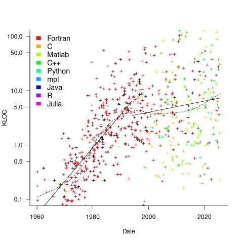
The two immediately obvious patterns are the sharp drop in the average rate of growth since the early 1990s (from 15% per year to 2% per year), and the dominance of Fortran until the early 2000s.
The growth in average implementation LOC might be caused by algorithms becoming more complicated, or because increasing computing resources meant that more code could be produced with the same amount of researcher effort, or another reason, or some combination. After around 2000, there is a significant increase in the variance in the size of implementations. I’m assuming that this is because some researchers focus on niche algorithms, while others continue to work on complicated algorithms.
An aim of Halstead’s early metric work was to create a measure of algorithm complexity.
If LLMs really do make researchers more productive, then in future years LOC growth rate should increase as more complicated problems are studied, or perhaps because LLMs generate more verbose code.
The table below shows the primary implementation language of the algorithm implementations:
  Language   Implementations
   Fortran        465
         C         79
    Matlab         72
       C++         24
    Python          7
         R          4
      Java          3
     Julia          2
MPL 1 |
If algorithms are becoming more complicated, then the papers describing/analysing them are likely to contain more pages. The plot below shows the number of pages in the published papers over time, with fitted regression line of the form  (0.38 pages per year; red dashed line is a LOESS regression model; code+data).
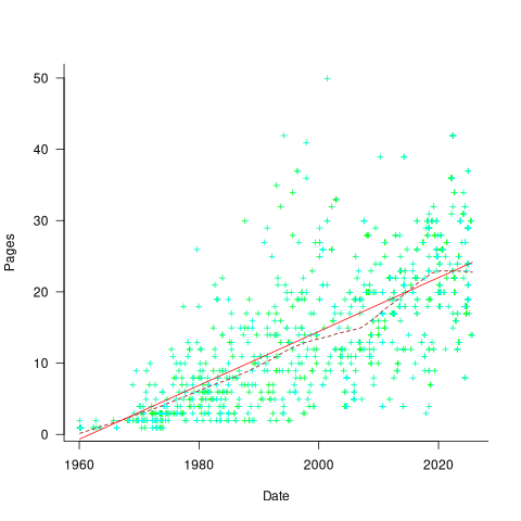
Unlike the growth of implementation LOC, there is no break-point in the linear growth of page count. Yes, page count is influence by factors such as long papers being less likely to be accepted, and being able to omit details by citing prior research.
It would be a waste of time to suggest more patterns of behavior without looking at a larger sample papers and their implementations (I have only looked at a handful).
When the source was distributed in several formats, the original one was used. Some algorithms came with build systems that included tests, examples and tutorials. The contents of the directories: CALGO_CD, drivers, demo, tutorial, bench, test, examples, doc were not counted.
Number of calls to/from functions vs function length
Depending on the language the largest unit of code is either a sequence of statements contained in a function/procedure/subroutine or a set of functions/methods contained in a larger unit, e.g., class/module/file. Connections between these largest units (e.g., calls to functions) provide a mechanism for analysing the structure of a program. These connections form a graph, and the structure is known as a call graph.
It is not always possible to build a completely accurate call graph by analysing a program’s source code (i.e., a static call graph) when the code makes use of function pointers. Uncertainty about which functions are called at certain points in the code is a problem for compiler writers wanting to do interprocedural flow analysis for code optimization, and static analysis tools looking for possible coding mistakes.
The following analysis investigates two patterns in the function call graph of C/C++ programs. While calls via function pointers can be very common at runtime, they are uncommon in the source. Function call information was extracted from 98 GitHub projects using CodeQL.
Functions that contain more code are likely to contain more function calls. The plot below shows lines of code against number of function calls for each of the 259,939 functions in whatever version of the Linux kernel is on GitHub today (25 Jan 2026), the red line is a regression fit showing  (the fit systematically deviates for larger functions {yet to find out why}; code and data):
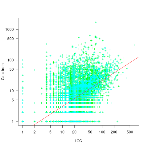
Researchers sometimes make a fuss of the fact that the number of calls per function is a power law, failing to note that this power law is a consequence of the number of lines per function being a power law (with an exponent of 2.8 for C, 2.7 for Java and 2.6 for Pharo). There are many small functions containing a few calls and a few large functions containing many calls.
Are more frequently called functions smaller (perhaps because they perform a simple operation that often needs to be done)? Widely used functionality is often placed in the same source file, and is usually called from functions in other files. The plot below shows the size of functions (in line of code) and the number of calls to them, for the 259,939 functions in the Linux kernel, with lines showing a LOESS fit to the corresponding points (code and data):
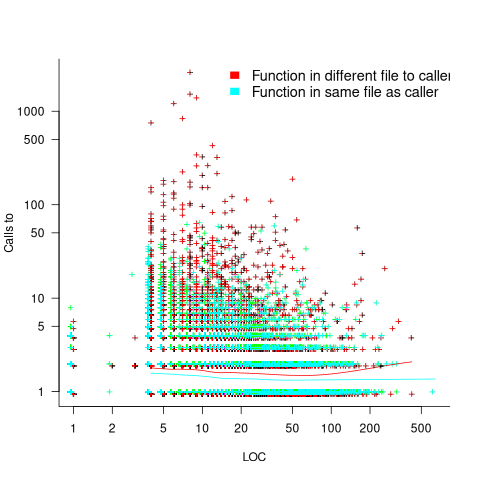
The apparent preponderance of red towards the upper left suggests that frequently called functions are short and contained in files different from the caller. However, the fitted LOESS lines show that the average difference is relatively small. There are many functions of a variety of sizes called once or twice, and few functions called very many times.
The program structure visible in a call graph is cluttered by lots of noise, such as calls to library functions, and the evolution baggage of previous structures. Also, a program may be built from source written in multiple languages (C/C++ is the classic example), and language interface issues can influence organization locally and globally (for instance, in Alibaba’s weex project the function main (in C) essentially just calls serverMain (in C++), which contains lots of code).
I suspect that many call graphs can be mapped to trees (the presence of recursion, though a chain of calls, sometimes comes as a surprise to developers working on a project). Call information needs to be integrated with loops and if-statements to figure out story structures (see section 6.9.1 of my C book). Don’t hold your breath for progress.
I expect that the above patterns are present in other languages. CodeQL supports multiple languages, but CodeQL source targeting one language has to be almost completely reworked to target another language, and it’s not always possible to extract exactly the same information. C/C++ appears have the best support.
Function calls are a component information
Modeling the distribution of method sizes
The number of lines of code in a method/function follows the same pattern in the three languages for which I have measurements: C, Java, Pharo (derived from Smalltalk-80).
The number of methods containing a given number of lines is a power law, with an exponent of 2.8 for C, 2.7 for Java and 2.6 for Pharo.
This behavior does not appear to be consistent with a simplistic model of method growth, in lines of code, based on the following three kinds of steps over a 2-D lattice: moving right with probability  , moving up and to the right with probability
  , and moving down and to the right with probability
  . The start of an
 if or for statement are examples of coding constructs that produce a step followed by a step at the end of the statement; steps are any non-compound statement. The image below shows the distinct paths for a method containing four statements:

For this model, if  the probability of returning to the origin after taking
  is a complicated expression with an exponentially decaying tail, and the case
  is a well studied problem in 1-D random walks (the probability of returning to the origin after taking steps is
  approx n^{-1.5}") ).
).
Possible changes to this model to more closely align its behavior with source statement production include:
- include terms for the correlation between statements, e.g., assigning to a local variable implies a later statement that reads from that variable,
- include context terms in the up/down probabilities, e.g., nesting level.
Measuring statement correlation requires handling lots of special cases, while measurements of up/down steps is easily obtained.
How can / probabilities be written such that step length has a power law with an exponent greater than two?
ChatGPT 5 told me that the Langevin equation and Fokker–Planck equation could be used to derive probabilities that produced a power law exponent greater than two. I had no idea had they might be used, so I asked ChatGPT, Grok, Deepseek and Kimi to suggest possible equations for the / probabilities.
The physics model corresponding to this code related problem involves the trajectories of particles at the bottom of a well, with the steepness of the wall varying with height. This model is widely studied in physics, where it is known as a potential well.
Reaching a possible solution involved refining the questions I asked, following suggestions that turned out to be hallucinations, and trying to work out what a realistic solution might look like.
One ChatGPT suggestion that initially looked promising used a Metropolis–Hastings approach, and a logarithmic potential well. However, it eventually dawned on me that ^a") , where
, where  is nesting level, and
  some constant, is unlikely to be realistic (I expect the probability of stepping up to decrease with nesting level).
Kimi proposed a model based on what it called algebraic divergence:
=r/{z(y)},U(y)={u_0y^{1-2/{alpha}}}/{z(y)}, D(y)={d_0y^{1-2/{alpha}}}/{z(y)}")
where: ") normalises the probabilities to equal one,
normalises the probabilities to equal one, =r+u_0y^{1-2/alpha}+d_0y^{1-2/alpha}") ,
,  is the up probability at nesting 0,
  is the down probability at nesting 0, and
  is the desired power law exponent (e.g., 2.8).
For C,  , giving
 =r/{z(y)},U(y)={u_0y^{0.29}}/{z(y)}, D(y)={d_0y^{0.29}}/{z(y)}")
The average length of a method, in LOC, is given by:
![E[LOC]={alpha r}/{2(d_0-u_0)}+O(e^{lambda}-1)](https://shape-of-code.com/wp-content/plugins/wpmathpub/phpmathpublisher/img/math_969.5_ffcacf0bb8190096d4d17fb475c0a290.png "E[LOC]={alpha r}/{2(d_0-u_0)}+O(e^{lambda}-1)") , where:
, where: }/{d_0+u_0}")
For C, the mean function length is 26.4 lines, and the values of  , , and need to be chosen subject to the constraint
  .
.
Combining the normalization factor with the requirement  , shows that as increases,
 ") slowly decreases and
slowly decreases and ") slowly increases.
slowly increases.
One way to judge how closely a model matches reality is to use it to make predictions about behavior patterns that were not used to create the model. The behavior patterns used to build this model were: function/method length is a power law with exponent greater than 2. The mean length, ![E[LOC]](https://shape-of-code.com/wp-content/plugins/wpmathpub/phpmathpublisher/img/math_981.5_0ac27fa76bd7c6e393f3497c9f30db7e.png "E[LOC]") , is a tuneable parameter.
, is a tuneable parameter.
Ideally a model works across many languages, but to start, given the ease of measuring C source (using Coccinelle), this one language will be the focus.
I need to think of measurable source code patterns that are not an immediate consequence of the power law pattern used to create the model. Suggestions welcome.
It’s possible that the impact of factors not included in this model (e.g., statement correlation) is large enough to hide any nesting related patterns that are there. While different kinds of compound statements (e.g., if vs. for) may have different step probabilities, in C, and I suspect other languages, if-statement use dominates (Table 1713.1: if 16%, for 4.6% while 2.1%, non-compound statements 66%).
Halstead/McCabe: a complicated formula for LOC
My experience is that people prefer to ignore the implications of Halstead’s metric and McCabe’s complexity metric being strongly correlated (non-linearly) with lines of code (LOC). The implications being that they have been deluding themselves and perhaps wasting time/money using Halstead/McCabe when they could just as well have used LOC.
If the purpose of collecting metrics is a requirement to tick a box, then it does not really matter which metrics are collected. The Halstead/McCabe metrics have a strong brand, so why not collect them.
Don’t make the mistake of thinking that Halstead/McCabe is more than a complicated way of calculating LOC. This can be shown by replacing Halstead/McCabe by the corresponding LOC value to find that it makes little difference to the value calculated.
Some metrics include the Halstead metrics and/or the McCabe metric as part of their calculation. The Maintainability Index is a metric calculated using Halstead’s volume, McCabe’s complexity and lines of code. Its equation is (see below for details):
-0.23*McCabe-16.2*ln(LOC)")
Replacing the Halstead/McCabe terms by one involving just LOC requires an appropriate mapping. Nearly all researchers assume a linear mapping, despite the overwhelming evidence that the mapping is non-linear.
Fitting regression models for HalsteadVolume vs LOC and McCabe vs LOC, using measurements of 730K methods from 47 Java projects (see below for data details), produces the coefficients for the equation needed to map each metric to LOC (previous analysis has found that a power law provides the best mapping; code+data). Substituting these equations in the Maintainability Index equation above, we get:
)-0.23*(0.45*LOC^{0.71})-16.2*ln(LOC)")
which simplifies to:
-0.1*LOC^{0.71}")
How does the value calculated using  compare with the corresponding
  value?
For 99.7% of methods, the relative error,  , for the 730K Java methods is less than 10%, and for 98.6% of methods the relative error is less than 5% (code+data).
Given the fuzzy nature of these metrics, 10% is essentially noise.
Looking at the relative contributions made by Halstead/McCabe/LOC to the value of the Maintainability Index, second equation above, the Halstead contribution is around a third the size of the LOC contribution and the McCabe contribution is at least an order of magnitude smaller.
Background on the Maintainability Index and the measured Java projects.
The Maintainability Index was introduced in the 1994 paper “Construction and Testing of Polynomials Predicting Software Maintainability” by Oman, and Hagemeister (270 citations; no online pdf), a 1992 paper by the same authors is often incorrectly cited (426 citations). The earlier 1992 paper identified 92 known maintainability attributes, along with 60 metrics for “… gauging software maintainability …” (extracted from 35 published papers).
This Maintainability Index equation was chosen from “Approximately 50 regression models were constructed and tested in our attempts to identify simple models that could be calculated from existing tools and still be generic enough to be applied to a wide range of software.” The data fitted came from eight suites of programs (average LOC 3,568 per suite), along “… with subjective engineering assessments of the quality and maintainability of each set of code.”
Yes, choosing from 50 regression models looks like overfitting, and by today’s standards 28.5K LOC is a tiny amount of source.
The data used is distributed with the paper Revisiting the Debate: Are Code Metrics Useful for Measuring Maintenance Effort? by Chowdhury, Holmes, Zaidman, and Kazman, which does a good job of outlining the many different definitions of maintenance and the inconsistent results from prediction models. However, the authors remain under the street light of project source code, i.e., they ignore the fact that many maintenance requests are driven by demand for new features.
The authors investigate the impact of normalizing Halstead/McCabe by LOC, but make the common mistake of assuming a linear relationship. They are surprised by the high correlation between post-‘normalised’ Halstead/McCabe and LOC. The correlation disappears when the appropriate non-linear normalization is used; see code+data.
A 2014 paper by Najm also maps the components of the Maintainability Index to LOC, but uses a linear mapping from the Halstead/McCabe terms to LOC, creating a equation whose behavior is noticeably different.
One code path dominates method execution
A recurring claim is that most reported faults are the result of coding mistakes in a small percentage of a program’s source code, with the 80/20 ‘rule’ being cited for social confirmation. I think there is something to this claim, but that the percentages are not so extreme.
A previous post pointed out that reported faults are caused by users. The 80/20 observation can be explained by users only exercising a small percentage of a program’s functionality (a tiny amount of data supports this observation). Surprisingly, there are researchers who believe that a small percentage of the code has some set of characteristics which causes it to contain most of a program’s coding mistakes (this belief has the advantage that a lot of source code is easily accessible and can be analysed to produce papers).
To what extent does user input direct program execution towards a small’ish subset of the code available to be executed?
The recent paper: Monitoring the Execution of 14K Tests: Methods Tend to Have One Path That Is Significantly More Executed by Andre Hora counted the number of times each path through a method’s source code was executed, when the method was called, for the 5,405 methods in 25 Python programs. These programs were driven by their 14,177 tests, rather than user input. The paper is focused on testing, in particular developer that developers tend to focus on positive tests.
Test suites are supposed to exercise all of a program’s source, so it is to be expected that these measurements will show a wider dispersion of code coverage than might be expected of typical user input.
The measurements also include a count of the lines executed/not executed along each executed method path. No information is provided on the number of unexecuted paths.
Within a method, there is always going to one path through the code that is executed more often than any other path. What this study found is that the most common path is often executed many more times than the other paths. The plot below shows, for each method (each +), the percentage of all calls to a method where the most common path was executed, against the total number of executed paths for that method; red/blue lines are fitted power law/exponential regression models, and the grey line shows the case where percentage executed is the fraction for a given number of paths (code+data):
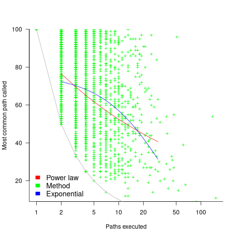
On average, the most common path is executed around four times more often than the second most commonly executed path.
While statistically significant, the fitted models do not explain much of the variance in the data. An argument can be made for either a power law and exponential distribution, and not having a feel for what to expect, I fitted both.
Non-error paths through a method have been found to be longer than the error paths. These measurements do not contain the information needed to attempt to replicate this finding.
New paths through a method are created by conditional statements, and the percentage of such statements in a method tends to be relatively constant across methods. The plot below shows the percentage of all calls to a method where the most common path was executed, where the method (each +) contains a given LOC; red/blue lines are fitted power law/exponential regression models (code+data):
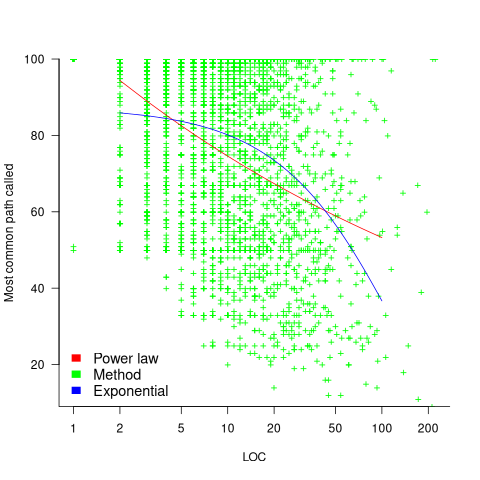
The models fitted to against LOC are better than those fitted against paths executed, but still not very good. A possible reason is that some methods will have unexecuted paths, LOC is a good proxy for total paths, and most common path percentage depends on total paths.
On average, 56% of a method’s LOC are executed along the most frequently executed path. When weighted by the number of method calls, the percentage is 48%.
The results of this study show that a call to most methods is likely to be dominated by the execution of one sequence of code. Another way that in which a small amount of code can dominate program execution is when most calls are to a small subset of the available methods. The plot below shows a density plot for the total number of calls to each method (code+data):

Around 62% of methods are called less than 100 times, while 2.6% are called over 10,000 times.
Small business programs: A dataset in the research void
My experience is that most of the programs created within organizations are very short, i.e., around 50–100 lines. Sometimes entire businesses are run using many short programs strung together in various ways. These short programs invariably make extensive use of the functionality provided by a much larger package that handles all the complicated stuff.
In the software development world, these short programs are likely to be shell scripts, but in the much larger ecosystem that is the business world these programs will be written in what used to be called a fourth generation language (4GL). These 4GLs are essentially domain specific languages for specific business tasks, such as report generation, or database query products, and for some time now spreadsheets.
The business software ecosystem is usually only studied by researchers in business schools, but short programs, business or otherwise, are rarely studied by any researchers. The source of such short programs is rarely publicly available; even if the information is not commercially confidential, the program likely addresses one group’s niche problem which is of no interest to anybody else, i.e., there is no rationale to publishing it. If source were available, there might not be enough of it to do any significant analysis.
I recently came across Clive Wrigley’s 1988 PhD thesis, which attempts to build a software estimation model. It contains summary data of 26 transaction processing systems written in the FOCUS language (an automated code generator).
For many organizations, there is a fundamental difference between business related problems and scientific/engineering problems, in that business problems tend to involve simple operations on lots of distinct data items (e.g., payroll calculation for each company employee), while scientific/engineering often involves a complicated formula operating on one set of data. There are exceptions.
4GLs enable technically proficient business users to create and maintain good enough applications without needing software engineering skills (yes, many do create spaghetti code), because they are not writing thousands of lines of code. The applications often contain many semi-self-contained subcomponents, which can be shared or swapped in/out. The small size makes it easier to change quickly, and there is direct access to the business users, it’s an agile process decades before this process took off in the world of non-4GL languages.
A major claim made by fans of 4GL is that it is much cheaper to create applications equivalent to those created using a 3GL, e.g., Cobol/C/C++/Java/Python/etc. I would agree that this true for small applications that fit the use-case addressed by a particular 4GL, but I think the domain specific nature of a 4GL will limit what can be done and likely need to be done in larger applications.
How do 4GL applications written in FOCUS compare against application written in Cobol? A 1987 paper by Chris Kemerer provides some manpower/LOC data for Cobol applications. I have no information on the amount of functionality in any of the applications. The plot below shows developer hours consumed creating 26 systems containing a given number of lines of code for FOCUS (green) and 15 COBOL (blue) programs, with fitted regression models in red (code+data):
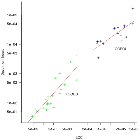
The two samples of applications differ by two orders of magnitude in LOC and developer hours, however, there is no information on the functionality provided by the applications.
Putnam’s software equation debunked
The implementation of a project has a lifecycle that starts and finishes with zero people working on it. Between starting and finishing, the number of staff quickly grows to a peak before slowly declining. In a series of very hard to obtain papers during the early 1960s (chapter 5), Peter Norden created a large project staffing model described by the Rayleigh equation. This model was evangelized by Lawrence Putnam in the 1970s, who called it the Norden/Rayleigh model, while others sometimes now call it the Norden/Putnam, Putnam/Rayleigh, or some combination of names; Putnam’s papers can be hard to obtain.
The Norden/Rayleigh equation is: 
where:  is work completed,
  is total manpower over the lifespan of the project,
  ,
,  is time of maximum effort per unit time (i.e., the Norden/Rayleigh equation maximum value, which Putnam calls project development time), and
  is project elapsed time.
Norden’s model is only applicable to large projects (e.g., 2+ man-years), and Putnam points out that the staffing of small projects is usually a square wave, i.e., a number of staff are allocated at the start and this number remains the same until project completion.
As well as evangelizing Norden’s model, Putnam also created his own model; an equation connecting delivered lines of code, total manpower and project duration. The usually cited paper for this work is: “A General Empirical Solution to the Macro Software Sizing and Estimating Problem”, which can sometimes be found as a free download. I had always assumed that people did not take this model seriously, and it was not worth my time debunking it. The paper makes conjures hand-wavy connections between various equations which don’t seem to go anywhere, and eventually connects together a regression equation fitted to nine data points with an observation+assumption about another regression equation to create what Putnam calls the software equation:  , where
  is delivered source code statements, and
  is a constant.
I recently read a 2014 paper by Han Suelmann debunking Putnam’s software equation, which led me to question my assumption about people not using Putnam’s model. Google Scholar shows 1,411 citations, with 133 since 2020. It looks like the software equation is still being taken seriously (or researchers are citing it because everybody else does; a common practice).
Why isn’t Putnam’s software equation worth treating seriously?
First, Putnam’s derivation of the software equation reads like a just-so story based on a tiny amount of data, and second a larger independent dataset does not show the pattern seen in Putnam’s data.
The derivation of the software equation starts by defining productivity as the number of delivered source code statements divided by the total manpower consumed to produce them,  . Ok.
. Ok.
There is more certainty to a line fitted to a set of points that roughly follow a straight line, than to fit a line to points that follow a curve (because there are usually many ‘curve’ equations to choose from). The Norden/Rayleigh equation can be transformed to a form that is amenable to fitting a straight line, i.e., dividing by time and taking logs, as follows (which plugs in the value of ):
=log(K/{t^2_d}) - (1/{2t^2_d})t^2")
Putnam noticed (or perhaps it was the authors of the cited prepublication paper “Software budgeting model” by G. E. P. Box and L. Pallesen, which I cannot locate a copy of) that when plotting ") against
against  : “If the number
  was small, it corresponded with easy systems; if the number was large, it corresponded with hard systems and appeared to fall in a range between these extremes.” Notice that in the screenshot of a figure from Putnam’s paper below, the y-axis is labelled “Difficulty”, not with the quantity actually plotted.
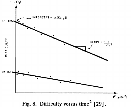
Based on an observation about easy/hard systems (it is never explained how easy/hard is measured) something called difficulty is defined to be:  . No explanation is given for dropping the log scaling, or the possibility that some other relationship might hold.
The screenshot below is of a figure from Putnam’s paper, which plots the values of against for 13 projects. The fitted regression lines (the three lines are fitted using, 9, 2 and 2 points of the 13 projects) have the form  , i.e.,
  (I extracted the points and fitted
  ; code+extracted data):
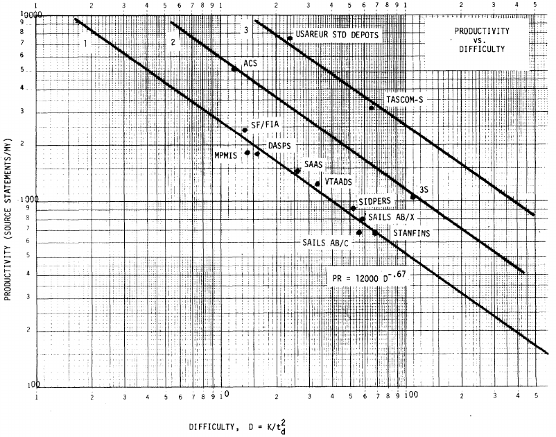
With a bit of algebra, the two equations: and , can be combined to create the software equation.
Yes, Putnam’s software equation was hand-waved into existence by plucking a “difficulty” component from an observation about the behavior of projects in a regression model and equating it to a regression line fitted to nine points.
Are the patterns seen by Putnam found in other projects?
In the 1987 paper “Time-Sensitive Cost Models in the Commercial MIS Environment” D. Ross Jeffery used data from 47 projects to investigate the effort/time relationships used by Putnam to derive his software equation.
The plot below, of log(Difficulty) vs log(Productivity), shows what appears to be a random scattering of points, confirmed by failing to fit a regression model (code+extracted data):

No. The patterns seen by Putnam are not present in these projects. I don’t think that the difference in application domain is relevant (Putnam’s projects were for Military systems and Jeffery’s are for commercial projects). Norden’s model is not specific to software projects.
Jeffery’s uses a regression model to find:  , the corresponding Putnam equation is:
 ^{-2/3}=C_2K^{-0.66}t^1.33_d") (the paper does not include the plot needed to extract the required data). The exponent might be claimed to be close enough, but the exponent is very different.
(the paper does not include the plot needed to extract the required data). The exponent might be claimed to be close enough, but the exponent is very different.
Jeffery’s paper includes a plot of ") against
against ") , and the plot below shows the extracted data (44 points), plus fitted regression line (code+extracted data):
, and the plot below shows the extracted data (44 points), plus fitted regression line (code+extracted data):
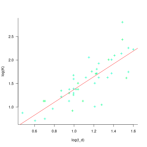
The regression line has the form  . This relationship further undermines assumptions made by Putnam, e.g., smaller systems are easier.
The Han Suelmann paper that triggered this post takes a very different approach to debunking Putnam’s model (he uses simulation to show that random data, drawn from a suitable distribution, can produce the patterns seen by Putnam).
Modeling program LOC growth with recurrence equations
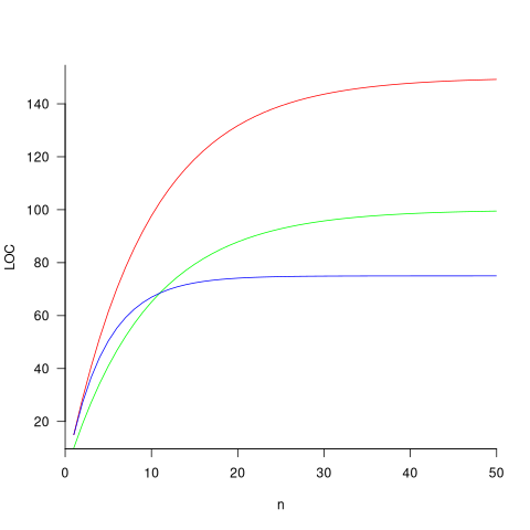
Models predicting the growth, in lines of code, of a program are based on the assumption that future growth follows the same pattern of behavior as past growth. One such model is the recurrence relation:
 , where:
  is LOC at time
  ,
,  is the LOC carried over from release , and
  is the LOC added after release .
The solution to this recurrence relation is: }/{1-a}+a^n*L_0") , where:
, where:  is the LOC at time
  .
.
The plot below shows the growth predicted by this model, for various values of and (code+data):
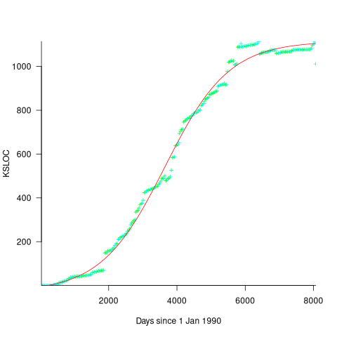
How close is the fit between this model and actual project growth? The plot below shows the growth in LOC for FreeBSD between 1993 and 2006, data from Herraiz; the red line shows the above equation fitted using non-linear regression, with the blue line showing a fitted linear regression model of the form  (code+data):
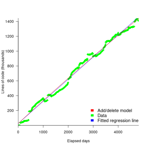
Plugging the fitted coefficients into the recurrence equation when  gives a prediction for the final maximum LOC in FreeBSD of:
}/{1-a} = 0.3124766/(1-0.9999750) = 12,477 KLOC")
The FreeBSD growth is unusual in not having a slow start to its growth, or rather no data is available prior to 1993.
Long-lived, successful projects usually attract new developers, and over time some developers leave. The size of a project, and the predispositions of those involved, can limit the number of active core developers. The above model can be applied to the growth in the number of active developers, i.e.,
 , where:
  is active developers at time ,
  is the developers ceasing to be active , and
  is the number of new active developers at . The solution is:
}/{1-c}+c^n*P_0")
Adding the developer growth equation in to the LOC model, we get:
 , where is now multiplied by the number of developers at time
  , i.e.,
  . The solution to these recurrence equations is somewhat involved (note: if you are using an LLM to check the answers, ChatGPT makes multiple mistakes, but the Grok response contains just one algebra mistake); when
  the equation is:
-d)/{c(1-c)}-b*d/{(1-c)(1-a)})*a^n+{b*(P_0*(1-c)-d)/{c(1-c)}}*c^{n-1}+b*d/{(1-c)(1-a)}")
Checking this more complicated model against another project, the plot below shows the growth of the GNU C library between 1990 and 2011, data from Gonzalez-Barahona, Robles, Herraiz and Ortega; the red line is the fitted equation /935}}") (code+data):
(code+data):
Unsurprisingly, I was not able to fit the more complicated growth model, using non-linear least squares, to the glibc LOC data. The problem was not being able to mimic the slow initial growth rate. I suspect that the developer growth model might be just wrong. Development work on a project does not last forever, and the number of developers will start decreasing at some point. For large projects, the Rayleigh distribution has been found to approximate staffing levels.
Data on project developer numbers over time is rare. The Linux kernel data shows an exponential developer growth rate, but I suspect that this is mostly caused by many one-time only developer contributing towards a new device driver (which are responsible for much of the Kernel growth).
Distribution of program sizes
Program size, in lines of code (LOC), used to be a topic of conversation among developers and managers. Program size is an issue when computer memory is measured in kilobytes. Large programs would be organized into overlays such that only small subsets needed to be held in memory at any time, i.e., programmer defined memory management.
Management used program size as a proxy for implementation effort/cost. Because size was a topic of conversation, it was possible to ask around to obtain a selection of values for the size of programs with similar functionality (accurate actual implementation costs were/are rarely available via the grapevine, but developers were/are always happy to talk about how small/large their programs were/are). These days, estimating LOC prior to implementation may appear more scientific, but I doubt it’s more accurate.
Once computers containing megabytes of memory became widespread, and the use of third-party libraries continued to grow, program size became a niche topic of conversation.
The size of some operating systems has become an occasional topic of conversation; it wasn’t previously because mainframe/mini computer manufacturers didn’t want customers talking about how much of their expensive memory was taken up by the OS. The size of Microsoft Windows leaked out and the Linux kernel is a topic of research.
Discussions around size have moved on from individual programs to the amount of space taken up by an installed application suite. Today, program size can be a rounding error compared to data files, extensions and add-ons.
Researchers have also moved on; repository size, in LOC/packages, is what now gets reported.
For those who are interested in program size; what is the distribution of program sizes? How many LOC are needed for a program to be above 50%, or in the top 95%?
Recent data on the size of individual programs is surprisingly hard to find, given how often LOC values appear in print. The one dataset I found is from the paper Empirical analysis of the relationship between CC and SLOC in a large corpus of Java methods and C functions, which is derived from the 2010’ish Sourcerer corpus of 13,103 Java projects (each of which I assume contains one program). The plot below shows the LOC (red) and methods (blue/green) for each program, in ascending order, along with values at various percentage points (code+data):
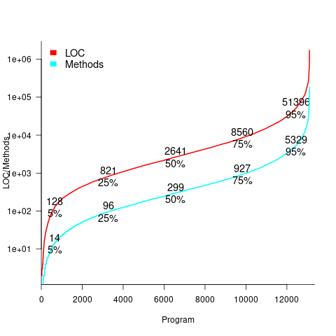
The size of Java programs is very likely to have increased since 2010. How much have grown? I don’t know.
What about the size of programs written in other languages?
I expect Python program size to be smaller, because the huge number of available package removes the need to implement a myriad of boilerplate functionality.
I expect C program size to be larger, both because of the smaller library ecosystem and because C programs tend to be older (programs rarely shrink with age).
Average lines added/deleted by commits across languages
Are programs written in some programming language shorter/longer, on average, than when written in other languages?
There is a lot of variation in the length of the same program written in the same language, across different developers. Comparing program length across different languages requires a large sample of programs, each implemented in different languages, and by many different developers. This sounds like a fantasy sample, given the rarity of finding the same specification implemented multiple times in the same language.
There is a possible alternative approach to answering this question: Compare the size of commits, in lines of code, for many different programs across a variety of languages. The paper: A Study of Bug Resolution Characteristics in Popular Programming Languages by Zhang, Li, Hao, Wang, Tang, Zhang, and Harman studied 3,232,937 commits across 585 projects and 10 programming languages (between 56 and 60 projects per language, with between 58,533 and 474,497 commits per language).
The data on each commit includes: lines added, lines deleted, files changed, language, project, type of commit, lines of code in project (at some point in time). The paper investigate bug resolution characteristics, but does not include any data on number of people available to fix reported issues; I focused on all lines added/deleted. Modifying a line will be treated as an deleted/added line.
Different projects (programs) will have different characteristics. For instance, a smaller program provides more scope for adding lots of new functionality, and a larger program contains more code that can be deleted. Some projects/developers commit every change (i.e., many small commit), while others only commit when the change is completed (i.e., larger commits). There may also be algorithmic characteristics that affect the quantity of code written, e.g., availability of libraries or need for detailed bit twiddling.
It is not possible to include project-id directly in the model, because each project is written in a different language, i.e., language can be predicted from project-id. However, program size can be included as a continuous variable (only one LOC value is available, which is not ideal).
The following R code fits a basic model (the number of lines added/deleted is count data and usually small, so a Poisson distribution is assumed; given the wide range of commit sizes, quantile regression may be a better approach):
alang_mod=glm(additions ~ language+log(LOC), data=lc, family="poisson") dlang_mod=glm(deletions ~ language+log(LOC), data=lc, family="poisson") |
Some of the commits involve tens of thousands of lines (see plot below). This sounds rather extreme. So two sets of models are fitted, one with the original data and the other only including commits with additions/deletions containing less than 10,000 lines.
These models fit the mean number of lines added/deleted over all projects written in a particular language, and the models are multiplicative. As expected, the variance explained by these two factors is small, at around 5%. The two models fitted are (code+data):
 or
or  , and
, and  or
or  , where the value of
  is listed in the following table, and
  is the number of lines of code in the project:
                    Original          0 < lines < 10000
    Language     Added     Deleted     Added   Deleted
    C              1.0       1.0         1.0     1.0
    C#             1.7       1.6         1.5     1.5
    C++            1.9       2.1         1.3     1.4
    Go             1.4       1.2         1.3     1.2
    Java           0.9       1.0         1.5     1.5
    Javascript     1.1       1.1         1.3     1.6
    Objective-C    1.2       1.4         2.0     2.4
    PHP            2.5       2.6         1.7     1.9
    Python         0.7       0.7         0.8     0.8
Ruby 0.3 0.3 0.7 0.7 |
These fitted models suggest that commit addition/deletion both increase as project size increases, by around  , and that, for instance, a commit in Go adds 1.4 times as many lines as C, and delete 1.2 as many lines (averaged over all commits). Comparing adds/deletes for the same language: on average, a Go commit adds
  lines, and deletes
  lines.
There is a strong connection between the number of lines added/deleted in each commit. The plot below shows the lines added/deleted by each commit, with the red line showing a fitted regression model  (code+data):
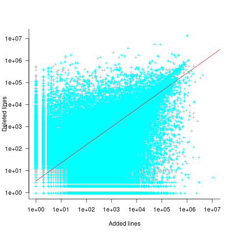
What other information can be included in a model? It is possible that project specific behavior(s) create a correlation between the size of commits; the algorithm used to fit this model assumes zero correlation. The glmer function, in the R package lme4, can take account of correlation between commits. The model component (language | project) in the following code adds project as a random effect on the language variable:
del_lmod=glmer(deletions ~ language+log(LOC)+(language | project), data=lc_loc, family=poisson) |
It takes around 24hr of cpu time to fit this model, which means I have not done much experimentation…
Recent Comments