Archive
Naming convergence in a network of pairwise interactions
While naming and categorizing things are perhaps the two most contentious issues in software engineering, there is often a great deal of similarity in the names and categorizes used by unconnected groups. These characteristics of naming and categorization are general observed behaviors across cultures and languages, with software engineering being a particular example.
Studies have found that a particular name for a thing is likely to become adopted by a group, if around 25% of its members actively promote the use of the name. The terms tipping point and critical mass have been applied to the 25% quantity.
What factors could cause 25% of the members of a group to select a particular name, and why does a tipping point occur at around this percentage?
The paper Experimental evidence for scale-induced category convergence across populations by Douglas Guilbeault (PhD thesis behind the paper), Andrea Baronchelli, and Damon Centola experimentally investigated factors that can cause a name to be adopted by 25% of a group’s members, and the researchers proposed a model that exhibits behavior similar to the experimental results (the supplement contains the technical details).
The experiment asked subjects to play the “Grouping Game”. The 1,480 online subjects were divided into networks containing either 2, 6, 8, 24 or 50 members. The interaction between members of a network only occurred via randomly selected pairs (the same pair for the network of two), with one person designated as the speaker and the other as the hearer. A pair saw three randomly selected images, such as the one below. For the speaker only, one of the images was highlighted, and they had to give a name containing at most six characters to the image. The hearer saw the name given by the speaker to one of the images, and had 30 seconds to choose the image they considered to have been named. If the image selected by the hearer was the one named by the speaker, both received a small payment, otherwise an even smaller amount was deducted from their final payment. Each subject played 100 rounds with the randomly chosen members of their network.

The images were created as a series of 50+ distinct patterns whose shape slowly morphed along a continuum, as in the following image:
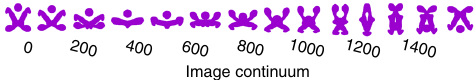
The experimental results were that larger networks converged to a consistent, within group, naming of the images (using a few names), while smaller groups rarely converged and used many different names. The researchers proposed that as the network size grew, common names were encountered more often than rarer names, increasing the likelihood of reaching a tipping point. This behavior is similar to the birthday paradox, where there is a 50% probability that in a room of 23 people, two people will share the same birthday.
In the experiment, some networks included confederates trained to use a small subset of names, i.e., the researchers created a common set of names. It was hypothesized built-in human preferences would produce common patterns in the real world that, for larger groups, would cause tipping points to occur, amplifying the more common patterns to become group norms.
The supplement to the paper develops a theoretical model based on the probability of  identical items being contained in a sample of
  items, when sampling without replacement. The solution involves the hypergeometric distribution, which is difficult to deal with analytically, so simulation is needed. The results show a tipping point at around 25%.
The plot below shows a density plot for one 50-subject network over 15 trials (after 100 rounds of pairwise interaction), with each color denoting one of the 14 chosen names (height of the curve denotes likelihood of the same name being chosen for that image; code and data):
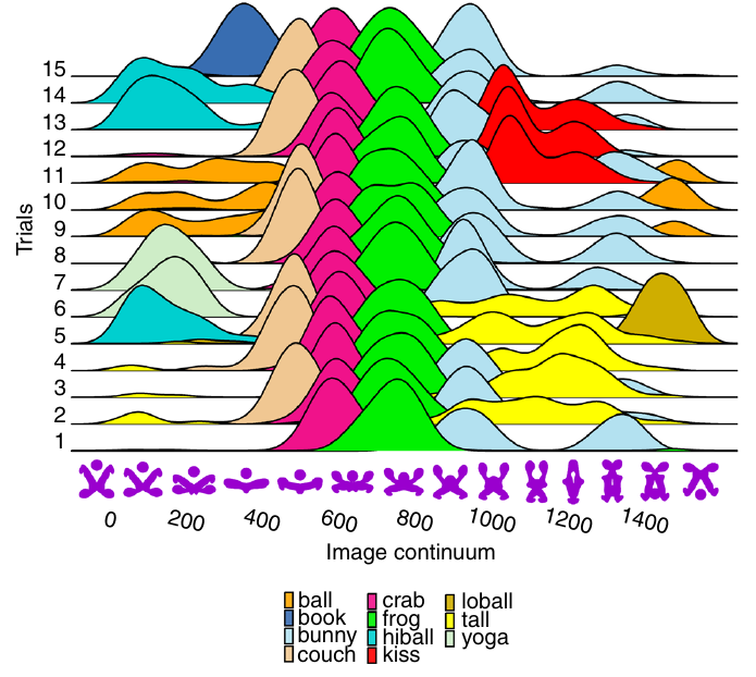
This plot shows that the same name is often used across trials, and naming boundaries between some images.
The plot below shows a density plot for one 2-subject network over 15 trials (after 100 rounds of pairwise interaction), with each color denoting one of the 72 chosen names (height of the curve denotes likelihood of the same name being chosen for that image; code and data):
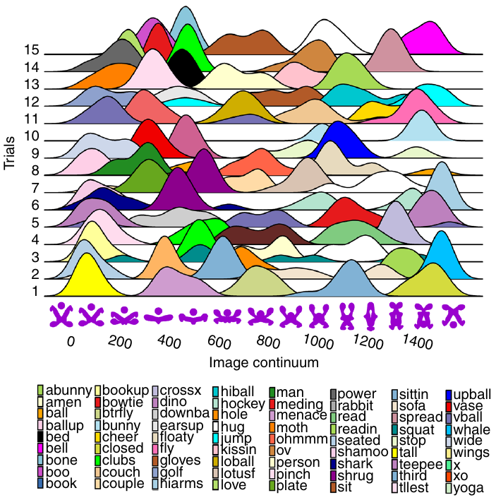
Here there is no consistent naming across trials, a much greater diversity of names appearing, and no obvious naming boundaries between images.
Impact of developer uncertainty on estimating probabilities
For over 50 years, it has been known that people tend to overestimate the likelihood of uncommon events/items occurring, and underestimate the likelihood of common events/items. This behavior has replicated in many experiments and is sometimes listed as a so-called cognitive bias.
Cognitive bias has become the term used to describe the situation where the human response to a problem (in an experiment) fails to match the response produced by the mathematical model that researchers believe produces the best output for this kind of problem. The possibility that the mathematical models do not reflect the reality of the contexts in which people have to solve the problems (outside of psychology experiments), goes against the grain of the idealised world in which many researchers work.
When models take into account the messiness of the real world, the responses are a closer match to the patterns seen in human responses, without requiring any biases.
The 2014 paper Surprisingly Rational: Probability theory plus noise explains biases in judgment by F. Costello and P. Watts (shorter paper), showed that including noise in a probability estimation model produces behavior that follows the human behavior patterns seen in practice.
If a developer is asked to estimate the probability that a particular event,  , occurs, they may not have all the information needed to make an accurate estimate. They may fail to take into account some s, and incorrectly include other kinds of events as being s. This noise,
  , introduces a pattern into the developer estimate:
*P_E + N*(1-P_E)=(1-2N)*P_E+N")
where:  is the developer’s estimated probability of event occurring,
  is the actual probability of the event, and is the probability that noise produces an incorrect classification of an event as
  or (for simplicity, the impact of noise is assumed to be the same for both cases).
The plot below shows actual event probability against developer estimated probability for various values of , with a red line showing that at  , the developer estimate matches reality (code):

The effect of noise is to increase probability estimates for events whose actually probability is less than 0.5, and to decrease the probability when the actual is greater than 0.5. All estimates move towards 0.5.
What other estimation behaviors does this noise model predict?
If there are two events, say  and
and  , then the noise model (and probability theory) specifies that the following relationship holds:
+P(B) == P(A & B)+P(A delim{|}{B}{})")
where: ") denotes the probability of its argument.
denotes the probability of its argument.
The experimental results show that this relationship does hold, i.e., the noise model is consistent with the experiment results.
This noise model can be used to explain the conjunction fallacy, i.e., Tversky & Kahneman’s famous 1970s “Lindy is a bank teller” experiment.
What predictions does the noise model make about the estimated probability of experiencing  (
( ) occurrences of the event in a sequence of
  assorted events (the previous analysis deals with the case
  )?
)?
An estimation model that takes account of noise gives the equation:

where:  is the developer’s estimated probability of experiencing s in a sequence of length , and
  is the actual probability of there being .
The plot below shows actual event probability against developer estimated probability for various values of , with a red line showing that at , the developer estimate matches reality (code):

This predicted behavior, which is the opposite of the case where , follows the same pattern seen in experiments, i.e., actual probabilities less than 0.5 are decreased (towards zero), while actual probabilities greater than 0.5 are increased (towards one).
There have been replications and further analysis of the predictions made by this model, along with alternative models that incorporate noise.
To summarise:
When estimating the probability of a single event/item occurring, noise/uncertainty will cause the estimated probability to be closer to 50/50 than the actual probability.
When estimating the probability of multiple events/items occurring, noise/uncertainty will cause the estimated probability to move towards the extremes, i.e., zero and one.
When task time measurements are not reported by developers
Measurements of the time taken to complete a software development task usually rely on the values reported by the person doing the work. People often give round number answers to numeric questions. This rounding has the effect of shifting start/stop/duration times to 5/10/15/20/30/45/60 minute boundaries.
To what extent do developers actually start/stop tasks on round number time boundaries, or aim to work for a particular duration?
The ABB Dev Interaction Data contains 7,812,872 interactions (e.g., clicking an icon) with Visual Studio by 144 professional developers performing an estimated 27,000 tasks over about 28,000 hours. The interaction start/stop times were obtained from the IDE to a 1-second resolution.
Completing a task in Visual Studio involves multiple interactions, and the task start/end times need to be extracted from each developer’s sequence of interactions. Looking at the data, rows containing the File.Exit message look like they are a reliable task-end delimiter (subsequent interactions usually happen many minutes after this message), with the next task for the corresponding developer starting with the next row of data.
Unfortunately, the time between two successive interactions is sometimes so long that it looks as if a task has ended without a File.Exit message being recorded. Plotting the number of occurrences of time-gaps between interactions (in minutes) suggests that it’s probably reasonable to treat anything longer than a 10-minute gap as the end of a task.
The plot below shows the number of tasks having a given duration, based on File.Exit, or using an 11-minute gap between interactions (blue/green) to indicate end-of-task, or a 20-minute gap (red; code+data):

The very prominent spikes in task counts at round numbers, seen in human reported times, are not present. The pattern of behavior is the same for both 11/20-minute gaps. I have no idea why there is a discontinuity at 10 minutes.
A development task is likely to involve multiple VS tasks. Is the duration of multiple VS tasks more likely to sum to a round number than a nonround number? There is no obvious reason why they should.
Is work on a VS task more likely to start/end at a round number time than a nonround number time?
Brief tasks are likely to be performed in the moment, i.e., without regard to clock time. Perhaps developers pay attention to clock time when tasks are expected to take some time.
The plot below shows the number of tasks taking at least 10-minutes that are started at a given number of minutes past the hour (blue/green), with red pluses showing 5-minute intervals (code+data):

No spikes in the count of tasks at round number start times (no spikes in the end times either; code+data).
Why spend time looking for round numbers where they are not expected to occur? Publishing negative results is extremely difficult, and so academics are unlikely to be interested in doing this analysis (not that software engineering researchers have shown any interest in round number usage).
Evolution has selected humans to prefer adding new features
Assume that clicking within any of the cells in the image below flips its color (white/green). Which cells would you click on to create an image that is symmetrical along the horizontal/vertical axis?

In one study, 80% of subjects added a block of four green cells in each of the three white corners. The other 20% (18 of 91 subjects) made a ‘subtractive’ change, that is, they clicked the four upper left cells to turn them white (code+data).
The 12 experiments discussed in the paper People systematically overlook subtractive changes by Adams, Converse, Hales, and Klotz (a replication) provide evidence for the observation that when asked to improve an object or idea, people usually propose adding something rather than removing something.
The human preference for adding, rather than removing, has presumably evolved because it often provides benefits that out weigh the costs.
There are benefits/costs to both adding and removing.
Creating an object:
- may produce a direct benefit and/or has the potential to increase the creator’s social status, e.g., ‘I made that’,
- incurs the cost of time and materials needed for the implementation.
Removing an object may:
- produce savings, but these are not always directly obvious, e.g., simplifying an object to reduce the cost of adding to it later. Removing (aka sacking) staff is an unpopular direct saving,
- generate costs by taking away any direct benefits it provides and/or reducing the social status enjoyed by the person who created it (who may take action to prevent the removal).
For low effort tasks, adding probably requires less cognitive effort than removing; assuming that removal is not a thoughtless activity. Chesterton’s fence is a metaphor for prudence decision-making, illustrating the benefit of investigating to find out if any useful service provided by what appears to be a useless item.
There is lots of evidence that while functionality is added to software systems, it is rarely removed. The measurable proxy for functionality is lines of code. Lots of source code is removed from programs, but a lot more is added.
Some companies have job promotion requirements that incentivize the creation of new software systems, but not their subsequent maintenance.
Open source is a mechanism that supports the continual adding of features to software, because it does not require funding. The C++ committee supply of bored consultants proposing new language features, as an outlet for their creative urges, will not dry up until the demand for developers falls below the supply of developers.
Update
The analysis in the paper More is Better: English Language Statistics are Biased Toward Addition by Winter, Fischer, Scheepers, and Myachykov, finds that English words (based on the Corpus of Contemporary American English) associated with an increase in quantity or number are much more common than words associated with a decrease. The following table is from the paper:
     Word       Occurrences
     add          361,246
     subtract       1,802
     addition      78,032
     subtraction      313
     plus         110,178
     minus         14,078
     more       1,051,783
     less         435,504
     most         596,854
     least        139,502
     many         388,983
     few          230,946
     increase      35,247
decrease 4,791 |
Software_Engineering_Practices = Morals+Theology
Including the word science in the term used to describe a research field creates an aura of scientific enterprise. Universities name departments “Computer Science” and creationist have adopted the term “Creation Science”. The word engineering is used when an aura with a practical hue is desired, e.g., “Software Engineering” and “Consciousness Engineering”.
Science and engineering theories/models are founded on the principle of reproducibility. A theory/model achieves its power by making predictions that are close enough to reality.
Computing/software is an amalgam of many fields, some of which do tick the boxes associated with science and/or engineering practices, e.g., the study of algorithms or designing hardware. Activities whose output is primarily derived from human activity (e.g., writing software) are bedevilled by the large performance variability of people. Software engineering is unlikely to ever become a real engineering discipline.
If the activity known as software engineering is not engineering, then what is it?
To me, software engineering appears to be a form of moral theology. My use of this term is derived from the 1988 paper Social Science as Moral Theology by Neil Postman.
Summarising the term moral theology via its two components, i.e., morality+theology, we have:
Morality is a system of rules that enable people to live and work together for mutual benefit. Social groups operate better when its members cooperate with each other based on established moral rules. A group operating with endemic within group lying and cheating is unlikely to survive for very long. People cannot always act selfishly, some level of altruism towards group members is needed to enable a group to flourish.
Development teams will perform better when its members cooperate with each other, as opposed to ignoring or mistreating each other. Failure to successfully work together increases the likelihood that the project the team are working on will failure; however, it is not life or death for those involved.
The requirements of group living, which are similar everywhere, produced similar moral systems around the world.
The requirements of team software development are similar everywhere, and there does appear to be a lot of similarity across recommended practices for team interaction (although I have not studied this is detail and don’t have much data).
Theology is the study of religious beliefs and practices, some of which do not include a god, e.g., Nontheism, Humanism, and Religious Naturalism.
Religious beliefs provide a means for people to make sense of their world, to infer reasons and intentions behind physical events. For instance, why it rains or doesn’t rain, or why there was plenty of animal prey during last week’s hunt but none today. These beliefs also fulfil various psychological and emotional wants or needs. The questions may have been similar in different places, but the answers were essentially invented, and so different societies have ended up with different gods and theologies.
Different religions do have some features in common, such as:
- Creation myths. In software companies, employees tell stories about the beliefs that caused the founders to create the company, and users of a programming language tell stories about the beliefs and aims of the language designer and the early travails of the language implementation.
- Imagined futures, e.g., we all go to heaven/hell: An imagined future of software developers is that source code is likely to be read by other developers, and code lives a long time. In reality, most source code has a brief and lonely existence.
A moral rule sometimes migrates to become a religious rule, which can slow the evolution of the rule when circumstances change. For instance, dietary restrictions (e.g., must not eat pork) are an adaptation to living in some environments.
In software development, the morals of an Agile methodology perfectly fitted the needs of the early Internet, where existing ways of doing things did not exist and nobody knew what customers really wanted. The signatories of the Agile manifesto now have their opinions treated like those of a prophet (these 17 prophets are now preaching various creeds).
Agile is not always the best methodology to use, with a Waterfall methodology being a better match for some environments.
Now that the Agile methodology has migrated to become a ‘religious’ dogma, the reaction to suggestions that an alternative methodology be used are often what one would expect to questioning a religious belief.
For me this is an evolving idea.
A surprising retrospective task estimation dataset
When estimating the time needed to implement a task, the time previously needed to implement similar tasks provides useful guidance. The implementation time for these previous tasks may itself be estimated, because the actual time was not measured or this information is currently unavailable.
How accurate are developer time estimates of previously completed tasks?
I am not aware of any software related dataset of estimates of previously completed tasks (it’s hard enough finding datasets containing information on the actual implementation time). However, I recently found the paper Dynamics of retrospective timing: A big data approach by Balcı, Ünübol, Grondin, Sayar, van Wassenhove, and Wittmann. The data analysed comes from a survey questionnaire, where 24,494 people estimated the how much time they had spent answering the questions, along with recording the current time at the start/end of the questionnaire. The supplementary data is in MATLAB format, and is also available as a csv file in the Blursday database (i.e., RT_Datasets).
Some of the behavior patterns seen in software engineering estimates appear to be general human characteristics, e.g., use of round numbers. An analysis of the estimation performance of a wide sample of the general population could help separate out characteristics that are specific to software engineering and those that apply to the general population.
The following table shows the percentage of answers giving a particular Estimate and Actual time, in minutes. Over 60% of the estimates are round numbers. Actual times are likely to be round numbers because people often give a round number when asked the time (code+data):
   Minutes    Estimate    Actual
     20          18%       8.5%
     15          15%       5.3%
     30          12%       7.6%
     25          10%       6.2%
10 7.7% 2.1% |
I was surprised to see that the authors had fitted a regression model with the Actual time as the explanatory variable and the Estimate as the response variable. The estimation models I have fitted always have the roles of these two variables reversed. More of this role reversal difference below.
The equation fitted to the data by the authors is (they use the term Elapsed, for consistency with other blog articles I continue to use Actual; code+data):

This equation says that, on average, for shorter Actual times the Estimate is higher than the Actual, while for longer Actual times the average Estimate is lower.
Switching the roles of the variables, I expected to see a fitted model whose coefficients are somewhat similar to the algebraically transformed version of this equation, i.e.,  . At the very least, I expected the exponent to be greater than one.
Surprisingly, the equation fitted with the variables roles reversed is very similar, i.e., the equations are the opposite of each other:

This equation says that, on average, for shorter Estimate times the Actual time is higher than the Estimate, while for longer Estimate times the average Actual is lower, i.e., the opposite behavior specifie dby the earlier equation.
I spent some time trying to understand how it was possible for data to be fitted such that (x ~ y) == (y ~ x), even posting a question to Cross Validated. I might, in a future post, discuss the statistical issues behind this behavior.
So why did the authors of this paper treat Actual as an explanatory variable?
After a flurry of emails with the lead author, Fuat Balcı (who was very responsive to my questions), where we both doubled checked the code/data and what we thought was going on, Fuat answered that (quoted with permission):
“The objective duration is the elapsed time (noted by the experimenter based on a clock reading), and the estimate is the participant’s response. According to the psychophysical approach the mapping between objective and subjective time can be defined by regressing the subjective estimates of the participants on the objective duration noted by the experimenter. Thus, if your research question is how human’s retrospective experience of time changes with the duration of events (e.g., biases in time judgments), the y-axis should be the participant’s response and the x-axis should be the actual duration.”
This approach has a logic to it, and is consistent with the regression modelling done by other researchers who study retrospective time estimation.
So which modelling approach is correct, and are people overestimating or underestimating shorter actual time durations?
Going back to basics, the structure of this experiment does not produce data that meets one of the requirements of the statistical technique we are both using (ordinary least squares) to fit a regression model. To understand why ordinary least squares, OLS, is not applicable to this data, it’s necessary to delve into a technical detail about the mathematics of what OLS does.
The equation actually fitted by OLS is:  , where
  is an error term (i.e., ‘noise’ caused by all the effects other than ). The value of is assumed to be exact, i.e., not contain any ‘noise’.
Usually, in a retrospective time estimation experiment, subjects hear, for instance, a sound whose duration is decided in advance by the experimenter; subjects estimate how long each sound lasted. In this experimental format, it makes sense for the Actual time to appear on the right-hand-side as an explanatory variable and for the Estimate response variable on the left-hand-side.
However, for the questionnaire timing data, both the Estimate and Actual time are decided by the person giving the answers. There is no experimenter controlling one of the values. Both the Estimate and Actual values contain ‘noise’. For instance, on a different day a person may have taken more/less time to actually answer the questionnaire, or provided a different estimate of the time taken.
The correct regression fitting technique to use is errors-in-variables. An errors-in-variables regression fits the equation:  + epsilon") , where:
, where:  is the true value of and
  is its associated error. A selection of packages are available for fitting a variety of errors-in-variables models.
I regularly see OLS used in software engineering papers (including mine) where errors-in-variables is the technically correct technique to use. Researchers are either unaware of the error issues or assuming that the difference is not important. The few times I have fitted an errors-in-variables model, the fitted coefficients have not been much different from those fitted by an OLS model; for this dataset the coefficient difference is obviously important.
The complication with building an errors-in-variables model is that values need to be specified for the error terms and . With OLS the value of is produced as part of the fitting process.
How might the required error values be calculated?
If some subjects round reported start/stop times, there may not be any variation in reported Actual time, or it may jump around in 5-minute increments depending on the position of the minute hand on the clock.
Learning researchers have run experiments where each subject performs the same task multiple times. Performance improves with practice, which makes it difficult to calculate the likely variability in the first-time performance. If we assume that performance is skill based, the standard deviation of all the subjects completing within a given timeframe could be used to calculate an error term.
With 60% of Estimates being round numbers, there might not be any variation for many people, or perhaps the answer given will change to a different round number. There is Estimate data for different, future tasks, and a small amount of data for the same future tasks. There is data from many retrospective studies using very short time intervals (e.g., tens of seconds), which might be applicable.
We could simply assume that the same amount of error is present in each variable. Deming regression is an errors-in-variables technique that supports this approach, and does not require any error values to be specified. The following equations have been fitted using Deming regression (code+data):

and

While these two equations are consistent with each other, we don’t know if the assumption of equal errors in both variables is realistic.
What next?
Hopefully it will be possible to work out reasonable error values for the Actual/Estimate times. Fitting a model using these values will tell us wether any over/underestimating is occurring, and the associated span of time durations.
I also need to revisit the analysis of software task estimation times.
What is known about software effort estimation in 2024
It’s three years since my 2021 post summarizing what I knew about estimating software tasks. While no major new public datasets have appeared (there have been smaller finds), I have talked to lots of developers/managers about the findings from the 2019/2021 data avalanche, and some data dots have been connected.
A common response from managers, when I outline the patterns found, is some variation of: “That sounds about right.” While it’s great to have this confirmation, it’s disappointing to be telling people what they already know, even if I can put numbers to the patterns.
Some of the developer behavior patterns look, to me, to be actionable, e.g., send developers on a course to unbias their estimates. In practice, managers are worried about upsetting developers or destabilising teams. It’s easy for an unhappy developer to find another job (the speakers at the meetups I attend often end by saying: “and we’re hiring.”)
This post summarizes a talk I gave recently on what is known about software estimating; a video will eventually appear on the British Computer Society‘s Software Practice Advancement group’s YouTube channel, and the slides are on Github.
What I call the historical estimation models contain source code, measured in lines, as a substantial component, e.g., COCOMO which overfits a miniscule dataset. The problem with this approach is that estimates of the LOC needed to implement some functionality LOC are very inaccurate, and different developers use different LOC to implement the same functionality.
Most academic research in software effort estimation continues to be based on miniscule datasets; it’s essentially fake research. Who is doing good research in software estimating? One person: Magne Jørgensen.
Almost all the short internal task estimate/actual datasets contain all the following patterns:
- use of round-numbers (known as heaping in some fields). The ratios of the most frequently used round numbers, when estimating time, are close to the ratios of the Fibonacci sequence,
- short tasks tend to be under-estimated and long tasks over-estimate. Surprisingly, the following equation is a good fit for many time-based datasets:
 ,
, - individuals tend to either consistently over or under estimate (this appears to be connected with the individual’s risk profile),
- around 30% of estimates are accurate, 68% within a factor of two, and 95% within a factor of four; one function point dataset, one story point dataset, many time datasets,
- developer estimation accuracy does not change with practice. Possible reasons for this include: variability in the world prevents more accurate estimates, developers choose to spend their learning resources on other topics (such as learning more about the application domain).
I have a new ChatGPT generated image for my slide covering the #Noestimates movement:

Motivation and software development
If people were not motivated to write software, computers would not have anything to do. What motivates a person to write software?
The source of human motivation may be intrinsic, as when pleasure is derived from performing the activity, or it may be extrinsic, such as being paid.
For some developers, writing software is a hedonistic activity. Intrinsic motivation continues to be the attractive force behind very many Open source projects.
People have to make a living, and being paid to write software creates an extrinsic motivation.
What do we know about human motivation?
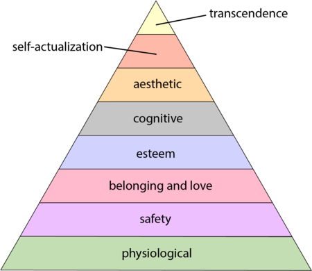
The 1943 paper A Theory of Human Motivation introduced Maslow’s hierarchy of needs, which is now often used as a structure for thinking about motivation. The image below, from Wikipedia, shows Maslow’s hierarchy:
Managers have long known that various kinds of carrots & sticks can be used to incentivize people to behave in a particular way, i.e., applying extrinsic motivation.
Incentives are actively researched in business and marketing departments. Unfortunately, sometimes more fashionable topics, such as cognitive biases, divert researcher’s interest.
Despite its fundamental importance, developer motivation is rarely considered, let alone a subject of research, within computing departments.
As purveyors of intangible goods, the software industry is aware of many issues around motivation. Managers of software teams appreciate the impact of team motivation on performance. Team motivation is a perennial topic of discussion for the Agile coaches and Scrum masters I meet. Companies selling products offering an API hire developer evangelists, whose job is to motivate third-party developers to use this API.
Software systems that continue to be used become part of the fabric of larger, more complex, systems. The motivations of the inhabitants of complex systems can have many unintended consequences.
Motivation is an intangible that cannot be measured directly; its effect has to be inferred from the results produced by the behaviors it drives. Distinguishing between two diametrically different motivations can present a conundrum, e.g., distinguishing between developers following Parkinson’s law or striving to meet a deadline.
Books don’t usually have much to say about the human side of software product management. A well-known exception is Peopleware: Productive Projects and Teams.
My evidence-based software engineering book should have had a chapter devoted to motivation, but given its focus on publicly available data, I had to make do with several 1-page subsections.
Printing press+widespread religious behavior: A theory
The book The Weirdest People in the World: How the West Became Psychologically Peculiar and Particularly Prosperous provides an explanation of the processes which weakened the existing social ties of family and tribe; however, the emergence of WEIRD people (Western, Educated, Industrialized, Rich and Democratic) required new social norms to spread and be accepted throughout society. A major technical innovation, in the form of the printing press, provided the means for mass communication of ideas and practices.
David High-Jones’ book Wyclif’s Dust: Western Cultures from the Printing Press to the Present describes the social consequences of what he calls book religion; a combination of deeply religious western societies and the ability of individuals to write and sell affordable books (made possible by the printing press). Religion+printing press created the conditions for what High-Jones calls a hothouse culture, a period from the 1600s to the end of the 1800s.
Around 1440 the printing press is invented and quickly spreads; around 5 million books were handwritten in the 1400s, about 80 million books were produced in the first 50 years of printing, and around a billion in the 1700s. During the 1500s the Protestant reformation happens; Protestant encouraged its followers to read the Bible, which creates a demand for printed Bibles and the need to be able to read (which increases literacy rates). In England, between 1480-1640, 40% of published books were religious.
The changes to society’s existing norms are wrought by cultural transmission, initially via middle class parents making use of edifying books to teach their children moral values and social skills, later Sunday schools took on this role, but also had to offer reading lessons to attract members. In the adult world, accepted norms were maintained by social enforcement. The impact on western societies was widespread because observant religious behavior was widespread.
The original intent, of those writing the religious books, was the creation of a god fearing society. In practice, a trust based society was created, where workers might be relied upon not to shirk their duties and businessmen to not renege on agreements.
In the beginning science, in the form of printed technical books, rarely made an appearance. In the 1700s the Enlightenment happens, and scientific books are discussed by small collections of disparate individuals. The industrial revolution happens, but the bulk of the demand is for trustworthy workers; technical and scientific know how remains a minority interest.
In Part I of the book, High-Jones weaves a reading and convincing narrative. Part II, 1900 to today, is a tale of the crumbling and breakdown of the social forces and incentives that creates the trust based society; while example are enumerated, no overarching theory is proposed (I skimmed this part).
Task backlog waiting times are power laws
Once it has been agreed to implement new functionality, how long do the associated tasks have to wait in the to-do queue?
An analysis of the SiP task data finds that waiting time has a power law distribution, i.e.,  , where
  is the number of tasks waiting a given amount of time; the LSST:DM Sprint/Story-point/Story has the same distribution. Is this a coincidence, or does task waiting time always have this form?
Queueing theory analyses the properties of systems involving the arrival of tasks, one or more queues, and limited implementation resources.
A basic result of queueing theory is that task waiting time has an exponential distribution, i.e., not a power law. What software task implementation behavior is sufficiently different from basic queueing theory to cause its waiting time to have a power law?
As always, my first line of attack was to find data from other domains, hopefully with an accompanying analysis modelling the behavior. It’s possible that my two samples are just way outside the norm.
Eventually I found an analysis of the letter writing response time of Darwin, Einstein and Freud (my email asking for the data has not yet received a reply). Somebody writes to a famous scientist (the scientist has to be famous enough for people to want to create a collection of their papers and letters), the scientist decides to add this letter to the pile (i.e., queue) of letters to reply to, eventually a reply is written. What is the distribution of waiting times for replies? Yes, it’s a power law, but with an exponent of -1.5, rather than -1.
The change made to the basic queueing model is to assign priorities to tasks, and then choose the task with the highest priority (rather than a random task, or the one that has been waiting the longest). Provided the queue never becomes empty (i.e., there are always waiting tasks), the waiting time is a power law with exponent -1.5; this behavior is independent of queue length and distribution of priorities (simulations confirm this behavior).
However, the exponent for my software data, and other data, is not -1.5, it is -1. A 2008 paper by Albert-László Barabási (detailed analysis) showed how a modification to the task selection process produces the desired exponent of -1. Each of the tasks currently in the queue is assigned a probability of selection, this probability is proportional to the priority of the corresponding task (i.e., the sum of the priorities/probabilities of all the tasks in the queue is assumed to be constant); task selection is weighted by this probability.
So we have a queueing model whose task waiting time is a power law with an exponent of -1. How well does this model map to software task selection behavior?
One apparent difference between the queueing model and waiting software tasks is that software tasks are assigned to a small number of priorities (e.g., Critical, Major, Minor), while each task in the model queue has a unique priority (otherwise a tie-break rule would have to be specified). In practice, I think that the developers involved do assign unique priorities to tasks.
Why wouldn’t a developer simply select what they consider to be the highest priority task to work on next?
Perhaps each developer does select what they consider to be the highest priority task, but different developers have different opinions about which task has the highest priority. The priority assigned to a task by different developers will have some probability distribution. If task priority assignment by developers is correlated, then the behavior is effectively the same as the queueing model, i.e., the probability component is supplied by different developers having different opinions and the correlation provides a clustering of priorities assigned to each task (i.e., not a uniform distribution).
If this mapping is correct, the task waiting time for a system implemented by one developer should have a power law exponent of -1.5, just like letter writing data.
The number of sprints that a story is assigned to, before being completely implemented, is a power law whose exponent varies around -3. An explanation of this behavior based on priority queues looks possible; we shall see…
The queueing models discussed above are a subset of the field known as bursty dynamics; see the review paper Bursty Human Dynamics for human behavior related aspects.
Recent Comments