Archive
Full Fact checking of number words
I was at the Full Fact hackathon last Friday (yes, a weekday hackathon; it looked interesting and interesting hackathons have been very thin on the ground in the last six months). Full Fact is an independent fact checking charity; the event was hosted by Facebook.
Full Fact are aiming to check facts in real-time, for instance tweeting information about inaccurate statements made during live political debates on TV. Real-time responses sounds ambitious, but they are willing to go with what is available, e.g., previously checked facts built up from intensive checking activities after programs have been aired.
The existing infrastructure is very basic, it is still early days.
Being a numbers person I volunteered to help out analyzing numbers. Transcriptions of what people say often contains numbers written as words rather than numeric literals, e.g., eleven rather than 11. Converting number words to numeric literals would enable searches to made over a range of values. There is an existing database of checked facts and Solr is the search engine used in-house, this supports numeric range searches over numeric literals.
Converting number words to numeric literals sounds like a common problem and I expected to be able to choose from a range of fancy Python packages (the in-house development language).
Much to my surprise, the best existing code I could find was rudimentary (e.g., no support for fractions or ranking words such as first, second).
spaCy was used to tokenize sentences and decide whether a token was numeric and text2num converted the token to a numeric literal (nltk has not kept up with advances in nlp).
I quickly encountered a bug in spaCy, which failed to categorize eighteen as a number word; an update was available on github a few hours after I reported the problem+fix :-). The fact that such an obvious problem had not been reported before suggests that few people are using this functionality.
Jenna, the other team member writing code, used beautifulsoup to extract sentences from the test data (formatted in XML).
Number words do not always have clear cut values, e.g., several thousand, thousands, high percentage and character sequences that could be dates. Then there are fraction words (e.g., half, quarter) and ranking words (e.g., first, second), all everyday uses that will need to be handled. It is also important to be able to distinguishing between dates, percentages and ‘raw’ numbers.
The UK is not the only country with independent fact checking organizations. A member of the Chequeado, in Argentina, was at the hack. Obviously number words will have to handle the conventions of other languages.
Full Fact are looking to run more hackathons in the UK. Keep your eyes open for Hackathon announcements. In the meantime, if you know of a good python library for handling word to number conversion, please let me know.
The future evolutionary cycle of application software?
At some time in the future (or perhaps it has already happened) all the features needed (by users) in a widely used application will have been implemented in that application. Once this point is reached, do the software developers involved go off and do something else (leaving a few behind to fix lingering faults)? This is not good news for software developers, perhaps they should continue adding features and hope that users don’t notice.
When the application is a commercial product there is every incentive for new releases to be driven by income from upgrades rather than user needs. When users stop paying for upgrades it is time to shift to renting the application in the cloud rather than selling licenses.
With an Open Source application most of the development may be funded commercially or may be funded by the enjoyment that the primary developers obtain from what they do. For renting to be a viable option, a major service components needs to be included, e.g., Github offers hosting along with the use of Git.
Halting development on commercial products is easy, it happens automatically when paying customers drop below the cost of development. Work on Open Source is not so easily halted. The enjoyment from writing software is does not rely on external funding, it is internally generated (having other people use your software is always a buzz and is a kind of external funding).
If the original core developers of an Open Source project move onto something else and nobody takes over, the code stops changing. However, this might only be the death of one branch, not the end of the road for development of what the application does. Eventually another developer decides it would be fun to reimplement the application in their favorite language. An example of this in Asciidoc (a document formatter), where the core developer decided to terminate personal involvement at the end of 2013 (a few people are making local updates to their own copies of the source, at least according to the Github fork timeline). Another developer appeared on the scene and decided to reimplement the functionality in Ruby, Asciidoctor.
Reimplementation of a tool in another language is a surprisingly common activity. There is a breed of developers who thinks that programs written in the language currently occupying their thoughts are magically better than the same program written in another language. At the moment Rust is an easy entanglement for those needing a language to love.
Over time, it will become harder and harder to install and run Asciidoc, because the ecosystem of libraries it depends on have evolved away from the behavior that is relied on. AsciiDoctor will become the default choice because it works on the available platforms. Eventually the core developer of AsciiDoctor will terminate his personal involvement; and then? Perhaps somebody will step forward to maintain the Ruby version or perhaps somebody will decide to reimplement in another language and around we go again.
The evolutionary cycle of software in the future is starting to look like it well be:
- developer(s) with enthusiasm and time on their hands, reimplement an application, (which is itself version n-1 of that application), in the language they love
- time passes and users accumulate, while the developer(s) actively supports application_n,
- those involved terminate involvement in supporting application_n,
- more time passes, during which the software ecosystem that applications+n depends on changes,
- successfully installing and running application_n is now so difficult that most users have migrated to application_(n+1).
Of course users will complain, but they don’t count in the world of Open Source (the role of users in Open Source is to provide adulation from which the core developers can extract sustenance).
Understanding where one academic paper fits in the plot line
Reading an academic paper is rather like watching an episode of a soap opera, unless you have been watching for a while you will have little idea of the roles played by the actors and the background to what is happening. A book is like a film in that it has a beginning-middle-end and what you need to know is explained.
Sitting next to somebody who has been watching for a while is a good way of quickly getting up to speed, but what do you do if no such person is available or ignores your questions?
How do you find out whether you are watching a humdrum episode or a major pivotal moment? Typing the paper’s title into Google, in quotes, can provide a useful clue; the third line of the first result returned will contain something like ’Cited by 219′ (probably a much lower number, with no ‘Cite by’ meaning ‘Cite by 0’). The number is a count of the other papers that cite the one searched on. Over 50% of papers are never cited and very recently published papers are too new to have any citations; a very few old papers accumulate thousands of citations.
Clicking on the ‘Cited by’ link will take you to Google Scholar and the list of later episodes involving the one you are interested in. Who are the authors of these later episodes (the names appear in the search results)? Have they all been written by the author of the original paper, i.e., somebody wandering down the street mumbling to himself? What are the citation counts of these papers? Perhaps the mumbler did something important in a later episode that attracted lots of attention, but for some reason you are looking at an earlier episode leading up to pivotal moment.
Don’t be put off by a low citation count. Useful work is not always fashionable and authors tend to cite what everybody else cites.
How do you find out about the back story? Papers are supposed to contain a summary of the back story of the work leading up to the current work, along with a summary of all related work. Page length restrictions (conferences invariably place a limit on the maximum length of a paper, e.g., 8 or 10 pages) mean that these summaries tend to be somewhat brief. The back story+related work summaries will cite earlier episodes, which you will then have to watch to find out a bit more about what is going on; yes, you guessed it, there is a rinse repeat cycle tracing episodes further and further back. If you are lucky you will find a survey article, which summarizes what is known based on everything that has been published up to a given point in time (in active fields surveys are published around every 10 years, with longer gaps in less active fields), or you will find the authors PhD thesis (this is likely to happen for papers published a few years after the PhD; a thesis is supposed to have a film-like quality to it and some do get published as books).
A couple of points about those citations you are tracing. Some contain typos (Google failing to return any matches for a quoted title is a big clue), some cite the wrong paper (invariable a cut-and-paste error by the author), some citations are only there to keep a referee happy (the anonymous people chosen to review a paper to decide whether it is worth publishing have been known to suggest their own work, or that of a friend be cited), some citations are only listed because everybody else cites them, and the cited work says the opposite of what everybody claims it says (don’t assume that just because somebody cites a paper that they have actually read it; the waterfall paper is the classic example of this).
After a week or two you should be up to speed on what is happening on the soap you are following.
Failed projects + the Cloud = Software reuse
Code reuse is one of those things that sounds like a winning idea to those outside of software development; those who write software for a living are happy to reuse other peoples’ code but don’t want the hassle involved with others reusing their own code. From the management point of view, where is the benefit in having your developers help others get their product out the door when they should be working towards getting your product out the door?
Lots of projects get canceled after significant chunks of software have been produced, some of it working. It would be great to get some return on this investment, but the likely income from selling software components is rarely large enough to make it worthwhile investing the necessary resources. The attractions of the next project are soon appear more enticing than hanging around baby-sitting software from a cancelled project.
Cloud services, e.g., AWS and Azure to name two, look like they will have a big impact on code reuse. The components of a failed project, i.e., those bits that work tolerably well, can be packaged up as a service and sold/licensed to other companies using the same cloud provider. Companies are already offering a wide variety of third-party cloud services, presumably the new software got written because no equivalent services was currently available on the provider’s cloud; well perhaps others are looking for just this service.
The upfront cost of sales is minimal, the services your failed re-purposed software provides get listed in various service directories. The software can just sit there waiting for customers to come along, or you could put some effort into drumming up customers. If sales pick up, it may become worthwhile offering support and even making enhancements.
What about the software built for non-failed projects? Software is a force multiplier and anybody working on a non-failed project wants to use this multiplier for their own benefit, not spend time making it available for others (I’m not talking about creating third-party APIs).
Is sorting a list of names racial discrimination?
Governments are starting to notice the large, and growing, role that algorithms have in the everyday life of millions of people. There is now an EU regulation, EU 2016/679, covering “… the protection of natural persons with regard to the processing of personal data…”
The wording in Article 22 has generated some waves: “The data subject shall have the right not to be subject to a decision based solely on automated processing, including profiling, which produces legal effects concerning him or her or similarly significantly affects him or her”
But I think something much bigger is tucked away in a subsection of Article 14 paragraph 2 “…the controller shall provide the data subject with the following information…”, subsection (g) “…meaningful information about the logic involved…” Explaining the program logic involved to managers who are supposed to have some basic ability for rational thought is hard enough, but the general public?
It is not necessary for the general public acquire a basic understanding of the logic behind some of the decisions made by computers, rabble-rousing by sections of the press and social media can have a big impact.
A few years ago I was very happy to see a noticeable reduction in my car insurance. This reduction was not the result of anything I had done, but because insurance companies were no longer permitted to discriminate on the basic of gender; men had previously paid higher car insurance premiums because the data showed they were a higher risk than women (who used to pay lower premiums). At last, some of the crazy stuff done in the name of gender equality benefited men.
Sorting would appear to be discrimination free, but ask any taxi driver about appearing first in a list of taxi phone numbers. Taxi companies are not called A1, AA, AAA because the owners are illiterate, they know all too well the power of appearing at the front of a list.
If you are in the market for a compiler writer whose surname starts with J (I have seen people make choices with less rationale than this), the following is obviously the most desirable expert listing (I don’t know any compiler writers called Kurt or Adalene):
Jones, Derek Jönes, Kurt Jônes, Adalene |
Now Kurt might object, pointing out that in German the letter ö is sorted as if it had been written oe, which means that Jönes gets to be sorted before Jones (in Estonian, Hungarian and Swedish, Jones appears first).
What about Adalene? French does not contain the letter ö, so who is to say she should be sorted after Kurt? Unicode specifies a collation algorithm, but we are in the realm of public opinion here, not having a techy debate.
This issue could be resolved in the UK by creating a brexit locale specifying that good old English letters always sort before Jonny foreigner letters.
Would use of such a brexit locale be permitted under EU 2016/679 (assuming the UK keeps this regulation), or would it be treated as racial discrimination?
I certainly would not want to be the person having to explain to the public the logic behind collation sequences and sort locales.
Automatically generated join-the-dots images
It is interesting to try and figure out what picture emerges from a join-the-dots puzzle (connect-the-dots in some parts of the world). Let’s have a go at some lightweight automatic generation such a puzzle (some heavy-weight techniques).
If an image is available, expressed as an boolean matrix, R’s sample function can be used to select a small percentage of the black points.
Taking the output of the following equation:
x=seq(-4.7, 4.7, by=0.002) y1 = c(1,-.7,.5)*sqrt(c(1.3, 2,.3)^2 - x^2) - c(.6,1.5,1.75) # 3 y2 =0.6*sqrt(4 - x^2)-1.5/as.numeric(1.3 <= abs(x)) # 1 y3 = c(1,-1,1,-1,-1)*sqrt(c(.4,.4,.1,.1,.8)^2 -(abs(x)-c(.5,.5,.4,.4,.3))^2) - c(.6,.6,.6,.6,1.5) # 5 y4 =(c(.5,.5,1,.75)*tan(pi/c(4, 5, 4, 5)*(abs(x)-c(1.2,3,1.2,3)))+c(-.1,3.05, 0, 2.6))/ as.numeric(c(1.2,.8,1.2,1) <= abs(x) & abs(x) <= c(3,3, 2.7, 2.7)) # 4 y5 =(1.5*sqrt(x^2 +.04) + x^2 - 2.4) / as.numeric(abs(x) <= .3) # 1 y6 = (2*abs(abs(x)-.1) + 2*abs(abs(x)-.3)-3.1)/as.numeric(abs(x) <= .4) # 1 y7 =(-.3*(abs(x)-c(1.6,1,.4))^2 -c(1.6,1.9, 2.1))/ as.numeric(c(.9,.7,.6) <= abs(x) & abs(x) <= c(2.6, 2.3, 2)) # 3 |
and sampling 300 of the 20,012 points we get images such as the following:

A relatively large sample size is needed to reduce the possibility that a random selection fails to return any points within a significant area, but we do end up with many points clustered here and there.
library("plyr")

rab_points=adply(x, 1, function(X) data.frame(x=rep(X, 18), y=c(
	c(1, -0.7, 0.5)*sqrt(c(1.3, 2, 0.3)^2-X^2) - c(0.6, 1.5 ,1.75),
	0.6*sqrt(4 - X^2)-1.5/as.numeric(1.3 <= abs(X)),
	c(1, -1, 1, -1, -1)*sqrt(c(0.4, 0.4, 0.1, 0.1, 0.8)^2-(abs(X)-c(0.5, 0.5, 0.4, 0.4, 0.3))^2) - c(0.6, 0.6, 0.6, 0.6, 1.5),
	(c(0.5, 0.5, 1, 0.75)*tan(pi/c(4, 5, 4, 5)*(abs(X)-c(1.2, 3, 1.2, 3)))+c(-0.1, 3.05, 0, 2.6))/
		as.numeric(c(1.2, 0.8, 1.2, 1) <= abs(X) & abs(X) <= c(3,3, 2.7, 2.7)),
	(1.5*sqrt(X^2+0.04) + X^2 - 2.4) / as.numeric(abs(X) <= 0.3),
	(2*abs(abs(X)-0.1)+2*abs(abs(X)-0.3)-3.1)/as.numeric(abs(X) <= 0.4),
	(-0.3*(abs(X)-c(1.6, 1, 0.4))^2-c(1.6, 1.9, 2.1))/
		as.numeric(c(0.9, 0.7, 0.6) <= abs(X) & abs(X) <= c(2.6, 2.3, 2))
						)))
rab_points$X1=NULL
rb=subset(rab_points, (!is.na(x)) & (!is.na(y) & is.finite(y)))

x=sample.int(nrow(rb), 300)
plot(rb$x[x], rb$y[x],
bty="n", xaxt="n", yaxt="n", pch=4, cex=0.5, xlab="", ylab="") |
A more uniform image can produced by removing all points less than a given distance from some selected set of points. In this case the point in the first element is chosen, everything close to it removed and the the processed repeated with the second element (still remaining) and so on.
rm_nearest=function(jp)
{
keep=((dot_im$x[(jp+1):(jp+window_size)]-dot_im$x[jp])^2+
      (dot_im$y[(jp+1):(jp+window_size)]-dot_im$y[jp])^2) < min_dist
keep=c(keep, TRUE) # make sure which has something to return
return(jp+which(keep))
}

window_size=500
cur_jp=1
dot_im=rb

while (cur_jp <= nrow(dot_im))
   {
#   min_dist=0.05+0.50*runif(window_size)
   min_dist=0.05+0.30*runif(1)
   dot_im=dot_im[-rm_nearest(cur_jp), ]
   cur_jp=cur_jp+1
   }

plot(dot_im$x, dot_im$y,
bty="n", xaxt="n", yaxt="n", pch=4, cex=0.5, xlab="", ylab="") |
Since R supports vector operations I want to do everything without using loops or if-statements. Yes, there is a while loop :-(, alternative, simple, non-loop suggestions welcome.
Removing points with an average squared distance less than 0.3 and 0.5 we get (with around 135-155 points) the images:

I was going to come up with a scheme for adding numbers, perhaps I will do this in another post.
Click for more equations generating images.
Christmas books for 2016
Here are couple of suggestions for books this Christmas. As always, the timing of the books I suggest is based on when they reach the top of the books-to-read pile, not when they were published.
“The Utopia of rules” by David Graeber (who also wrote the highly recommended “Debt : The First 5000 Years”). Full of eye opening insights into bureaucracy, how the ‘free’ world’s state apparatus came to have its current form and how various cultures have reacted to the imposition of bureaucratic rules. Very readable.
“How Apollo Flew to the Moon” by W. David Woods. This is a technical nuts-and-bolts story of how Apollo got to the moon and back. It is the best book I have every read on the subject, and as a teenager during the Apollo missions I read all the books I could find.
This year’s blog find was Scott Adams’ blog (yes, he of Dilbert fame). I had been watching Donald Trump’s rise for about a year and understood that almost everything he said was designed to appeal to a specific audience and the fact that it sounded crazy to those not in the target audience was irrelevant. I found Scott’s blog contained lots of interesting insights of the goings on in the US election; the insights into why Trump was saying the things he said have proved to be spot on.
For those of you interested in theoretical physics I ought to mention Backreaction (regular updates, primarily about gravity related topics) and Of Particular Significance (sporadic updates and primarily about particle physics)
Giving engineers the freedom to create a customer lock-in Cloud
The Cloud looks like the next dominant platform for hosting applications.
What can a Cloud vendor do to lock customers in to their fluffy part of the sky?
I think that Microsoft showed the way with their network server protocols (in my view this occurred because of the way things evolved, not though any cunning plan for world domination). The EU/Microsoft judgment required Microsoft to document and license their server protocols; the purpose was to allow third-parties to product Microsoft server plug-compatible products. I was an advisor to the Monitoring trustee entrusted with monitoring Microsoft’s compliance and got to spend over a year making sure the documents could be implemented.
Once most the protocol documents were available in a reasonably presentable state (Microsoft originally considered the source code to be the documentation and even offered it to the EU commission to satisfy the documentation requirement; they eventually hire a team of several hundred to produce prose specifications), two very large hurdles to third party implementation became apparent:
- the protocols were a tangled mess of interdependencies; 100% compatibility required implementing all of them (a huge upfront cost),
- the specification of the error behavior (i.e., what happens when something goes wrong) was minimal, e.g., when something unexpected occurs one of the errors in
windows.his returned (when I last checked, 10 years ago, this file contained over 30,000 identifiers).
Third party plugins for Microsoft server protocols are not economically viable (which is why I think Microsoft decided to make the documents public, they had nothing to loose and could claim to be open).
A dominant cloud provider has the benefit of size, they have a huge good-enough code base. A nimbler, smaller, competitor will be looking for ways to attract customers by offering a better service in some area, which means finding a smaller, stand-alone, niche where they can add value. Widespread use of Open Source means everybody gets to see and use most of the code. The way to stop smaller competitors gaining a foothold is to make sure that the code hangs together as a whole, with no relatively stand-alone components that can be easily replaced. Mutual interdependencies and complexity creates a huge barrier to new market entrants and is in the best interests of dominant vendors (yes it creates extra costs for them, but these are the price for detering competitors).
Engineers will create intendependencies between components and think nothing of it; who does not like easy solutions to problems and this one dependency will not hurt will it? Taking the long term view, and stopping engineers taking short cuts for short term gain, requires a lot of effort; who could fault a Cloud vendor for allowing mutual interdependencies and complexity to accumulate over time.
Error handling is a very important topic that rarely gets the attention it deserves, nobody likes to talk about the situation where things go wrong. Error handling is the iceberg of application development, while the code is often very mundane, its sheer volume (it can be 90% of the code in an application) creates a huge lock-in. The circumstances under which a system handles raises an error and the feasible recovery paths are rarely documented in any detail, it is something that developers working at the coal face learn by trial and error.
Any vendor looking to poach customers first needs to make sure they don’t raise any errors that the existing application does not handle and second any errors they do raise need to be solvable using the known recovery paths. Even if there is error handling information available to enable third-parties to duplicate responses, the requirement to duplicate severely hampers any attempt to improve on what already exists (apart from not raising the errors in the first place).
To create an environment for customer lock-in, Cloud vendors need to encourage engineers to keep doing what engineers love to do: adding new features and not worrying about existing spaghetti code.
Ability to remember code improves with experience
What mental abilities separate an expert from a beginner?
In the 1940s de Groot studied expertise in Chess. Players were shown a chess board containing various pieces and then asked to recall the locations of the pieces. When the location of the chess pieces was consistent with a likely game, experts significantly outperformed beginners in correct recall of piece location, but when the pieces were placed at random there was little difference in recall performance between experts and beginners. Also players having the rank of Master were able to reconstruct the positions almost perfectly after viewing the board for just 5 seconds; a recall performance that dropped off sharply with chess ranking.
The interpretation of these results (which have been duplicated in other areas) is that experts have learned how to process and organize information (in their field) as chunks, allowing them to meaningfully structure and interpret board positions; beginners don’t have this ability to organize information and are forced to remember individual pieces.
In 1981 McKeithen, Reitman, Rueter and Hirtle repeated this experiment, but this time using 31 lines of code and programmers of various skill levels. Subjects were given two minutes to study 31 lines of code, followed by three minutes to write (on a blank sheet of paper) all the code they could recall; this process was repeated five times (for the same code). The plot below shows the number of lines correctly recalled by experts (2,000+ hours programming experience), intermediates (just finished programming course) and beginners (just started programming course), left performance using ‘normal’ code and right is performance viewing code created by randomizing lines from ‘normal’ code; only the mean values in each category are available (code+data):
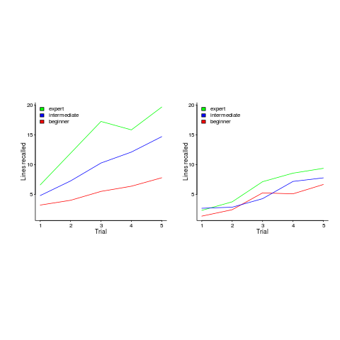
Experts start off remembering more than beginners and their performance improves faster with practice.
Compared to the Power law of practice (where experts should not get a lot better, but beginners should improve a lot), this technique is a much less time consuming way of telling if somebody is an expert or beginner; it also has the advantage of not requiring any application domain knowledge.
If you have 30 minutes to spare, why not test your ‘expertise’ on this code (the .c file, not the .R file that plotted the figure above). It’s 40 odd lines of C from the Linux kernel. I picked C because people who know C++, Java, PHP, etc should have no trouble using existing skills to remember it. What to do:
- You need five blank sheets of paper, a pen, a timer and a way of viewing/not viewing the code,
- view the code for 2 minutes,
- spend 3 minutes writing down what you remember on a clean sheet of paper,
- repeat until done 5 times.
Count how many lines you correctly wrote down for each iteration (let’s not get too fussed about exact indentation when comparing) and send these counts to me (derek at the primary domain used for this blog), plus some basic information on your experience (say years coding in language X, years in Y). It’s anonymous, so don’t include any identifying information.
I will wait a few weeks and then write up the data o this blog, as well as sharing the data.
Update: The first bug in the experiment has been reported. It takes longer than 3 minutes to write out all the code. Options are to stick with the 3 minutes or to spend more time writing. I will leave the choice up to you. In a test situation, maximum time is likely to be fixed, but if you have the time and want to find out how much you remember, go for it.
Uncertainty in data causes inconsistent models to be fitted
Does software development benefit from economies of scale, or are there diseconomies of scale?
This question is often expressed using the equation:  . If
. If  is less than one there are economies of scale, greater than one there are diseconomies of scale. Why choose this formula? Plotting project effort against project size, using logs scales, produces a series of points that can be sort-of reasonably fitted by a straight line; such a line has the form specified by this equation.
Over the last 40 years, fitting a collection of points to the above equation has become something of a rite of passage for new researchers in software cost estimation; values for have ranged from 0.6 to 1.5 (not a good sign that things are going to stabilize on an agreed value).
This article is about the analysis of this kind of data, in particular a characteristic of the fitted regression models that has been baffling many researchers; why is it that the model fitted using the equation is not consistent with the model fitted using  , using the same data. Basic algebra requires that the equality
  be true, but in practice there can be large differences.
The data used is Data set B from the paper Software Effort Estimation by Analogy and Regression Toward the Mean (I cannot find a pdf online at the moment; Code+data). Another dataset is COCOMO 81, which I analysed earlier this year (it had this and other problems).
The difference between and  is a result of what most regression modeling algorithms are trying to do; they are trying to minimise an error metric that involves just one variable, the response variable.
In the plot below left a straight line regression has been fitted to some Effort/Size data, with all of the error assumed to exist in the  values (dotted red lines show the residual for each data point). The plot on the right is another straight line fit, but this time the error is assumed to be in the
  values (dotted green lines show the residual for each data point, with red line from the left plot drawn for reference). Effort is measured in hours and Size in function points, both scales show the
  of the actual value.
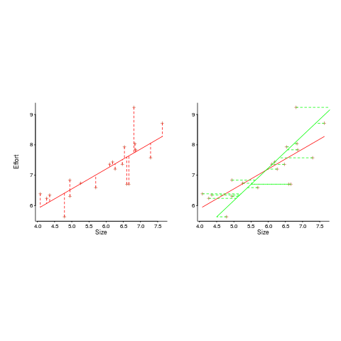
Regression works by assuming that there is NO uncertainty/error in the explanatory variable(s), it is ALL assumed to exist in the response variable. Depending on which variable fills which role, slightly different lines are fitted (or in this case noticeably different lines).
Does this technical stuff really make a difference? If the measurement points are close to the fitted line (like this case), the difference is small enough to ignore. But when measurements are more scattered, the difference may be too large to ignore. In the above case, one fitted model says there are economies of scale (i.e.,  ) and the other model says the opposite (i.e.,
  , diseconomies of scale).
There are several ways of resolving this inconsistency:
- conclude that the data contains too much noise to sensibly fit a a straight line model (I think that after removing a couple of influential observations, a quadratic equation might do a reasonable job; I know this goes against 40 years of existing practice of do what everybody else does…),
- obtain information about other important project characteristics and fit a more sophisticated model (characteristics of one kind or another are causing the variation seen in the measurements). At the moment information is being used to explain all of the variance in the data, which cannot be done in a consistent way,
- fit a model that supports uncertainty/error in all variables. For these measurements there is uncertainty/error in both and ; writing the same software using the same group of people is likely to have produced slightly different Effort/Size values.
There are regression modeling techniques that assume there is uncertainty/error in all variables. These are straight forward to use when all variables are measured using the same units (e.g., miles, kilogram, etc), but otherwise require the user to figure out and specify to the model building process how much uncertainty/error to attribute to each variable.
In my Empirical Software Engineering book I recommend using simex. This package has the advantage that regression models can be built using existing techniques and then ‘retrofitted’ with a given amount of standard deviation in specific explanatory variables. In the code+data for this problem I assumed 10% measurement uncertainty, a number picked out of thin air to sound plausible (its impact is to fit a line midway between the two extremes seen in the right plot above).
Recent Comments