Archive
Number of calls to/from functions vs function length
Depending on the language the largest unit of code is either a sequence of statements contained in a function/procedure/subroutine or a set of functions/methods contained in a larger unit, e.g., class/module/file. Connections between these largest units (e.g., calls to functions) provide a mechanism for analysing the structure of a program. These connections form a graph, and the structure is known as a call graph.
It is not always possible to build a completely accurate call graph by analysing a program’s source code (i.e., a static call graph) when the code makes use of function pointers. Uncertainty about which functions are called at certain points in the code is a problem for compiler writers wanting to do interprocedural flow analysis for code optimization, and static analysis tools looking for possible coding mistakes.
The following analysis investigates two patterns in the function call graph of C/C++ programs. While calls via function pointers can be very common at runtime, they are uncommon in the source. Function call information was extracted from 98 GitHub projects using CodeQL.
Functions that contain more code are likely to contain more function calls. The plot below shows lines of code against number of function calls for each of the 259,939 functions in whatever version of the Linux kernel is on GitHub today (25 Jan 2026), the red line is a regression fit showing  (the fit systematically deviates for larger functions {yet to find out why}; code and data):
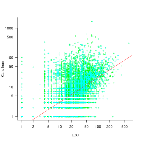
Researchers sometimes make a fuss of the fact that the number of calls per function is a power law, failing to note that this power law is a consequence of the number of lines per function being a power law (with an exponent of 2.8 for C, 2.7 for Java and 2.6 for Pharo). There are many small functions containing a few calls and a few large functions containing many calls.
Are more frequently called functions smaller (perhaps because they perform a simple operation that often needs to be done)? Widely used functionality is often placed in the same source file, and is usually called from functions in other files. The plot below shows the size of functions (in line of code) and the number of calls to them, for the 259,939 functions in the Linux kernel, with lines showing a LOESS fit to the corresponding points (code and data):
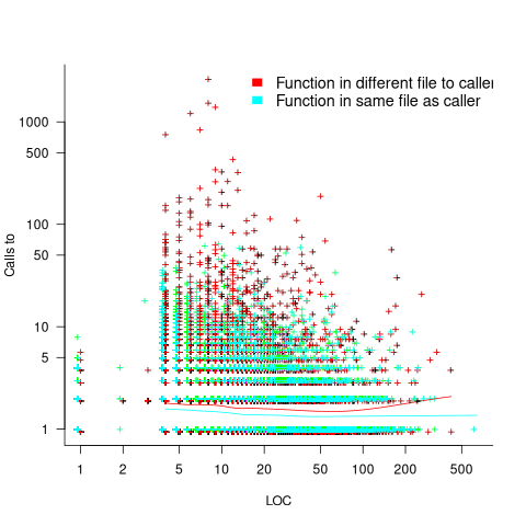
The apparent preponderance of red towards the upper left suggests that frequently called functions are short and contained in files different from the caller. However, the fitted LOESS lines show that the average difference is relatively small. There are many functions of a variety of sizes called once or twice, and few functions called very many times.
The program structure visible in a call graph is cluttered by lots of noise, such as calls to library functions, and the evolution baggage of previous structures. Also, a program may be built from source written in multiple languages (C/C++ is the classic example), and language interface issues can influence organization locally and globally (for instance, in Alibaba’s weex project the function main (in C) essentially just calls serverMain (in C++), which contains lots of code).
I suspect that many call graphs can be mapped to trees (the presence of recursion, though a chain of calls, sometimes comes as a surprise to developers working on a project). Call information needs to be integrated with loops and if-statements to figure out story structures (see section 6.9.1 of my C book). Don’t hold your breath for progress.
I expect that the above patterns are present in other languages. CodeQL supports multiple languages, but CodeQL source targeting one language has to be almost completely reworked to target another language, and it’s not always possible to extract exactly the same information. C/C++ appears have the best support.
Function calls are a component information
Formal methods and LLM generated mathematical proofs
Formal methods have been popping up in the news again, or at least on the technical news sites I follow.
Both mathematics and software share the same pattern of usage of formal methods. The input text is mapped to some output text. Various characteristics of the output text are checked using proof assistant(s). Assuming the mapping from input to output is complete and accurate, and the output has the desired characteristics, various claims can then be made about the input text, e.g., internally consistent. For software systems, some of the claims of correctness made about so-called formally verified systems would make soap powder manufacturers blush.
Mathematicians have been using LLMs to help find proofs of unsolved maths problems. Human written proofs are traditionally checked by other humans reading them to verify that the claimed proof is correct. LLMs generated proofs are sometimes written in what is called a formal language, this proof-as-program can then be independently checked by a proof assistant (the Lean proof assistant is a popular choice; Rocq is popular for proofs about software).
Software developers are well aware that LLM generated code contains bugs, and mathematicians have discovered that LLM generated proof-programs contain bugs. A mathematical proof bug involves Lean reporting that the LLM generated proof is true, when the proof applies to a question that is different from the actual question asked. Developers have probably experienced the case where an LLM generates a working program that does not do what was requested.
An iterative verification-and-refinement pipeline was used for LLMs well publicised solving of International Mathematical Olympiad problems.
A cherished belief of fans of formal methods is that mathematical proofs are correct. Experience with LLMs shows that a sequence of steps in a generated proof may be correct, but the steps may go down a path unrelated to the question posed in the input text. Also, proof assistants are programs, and programs invariably contain coding mistakes, which sometimes makes it possible to prove that false is true (one proof assistant currently has 83 bug reports of false being proved true).
It is well known, at least to mathematicians, that many published proofs contain mistakes, but that these can be fixed (not always easily), and the theorem is true. Unfortunately, journals are not always interested in publishing corrections. A sample of 51 reviews of published proofs finds that around a third contain serious errors, not easily corrected.
Human written proofs contain intentional gaps. For instance, it is assumed that readers can connect two steps without more details being given, or the author does not want to deter reviewers with an overly long proof. If LLM generated proofs are checked by proof assistants, then the gap between steps needs to be of a size supported by the assistant, and deterring reviewers is not an issue. Does this mean that LLM generated proof is likely to be human unfriendly?
Software is often expressed in an imperative language, which means it can be executed and the output checked. Theorems in mathematics are often expressed in a declarative form, which makes it difficult to execute a theorem to check its output.
For software systems, my view is that formal methods are essentially a form of  -version programming, with
  . Two programs are written, with one nominated to be called the specification; one or more tools are used to analyse both programs, checking that their behavior is consistent, and sometimes other properties. Mistakes may exist in the specification program or the non-specification program.
Using LLMs to help solve mathematical problems is a rapidly evolving field. We will have to wait and see whether end-to-end LLM generated proofs turn out to be trustworthy, or remain as a very useful aid.
Distribution of small project completion times
Records of project estimates and actual task times show that round numbers are very common. Various possible reasons have been suggested for why actual times are often reported as a round number. This post analyses the impact of round number reports of actual times on the accuracy of estimates.
The plot below shows the number of tasks having a given reported completion time for 1,525 tasks estimated to take 1-hour (code+data):
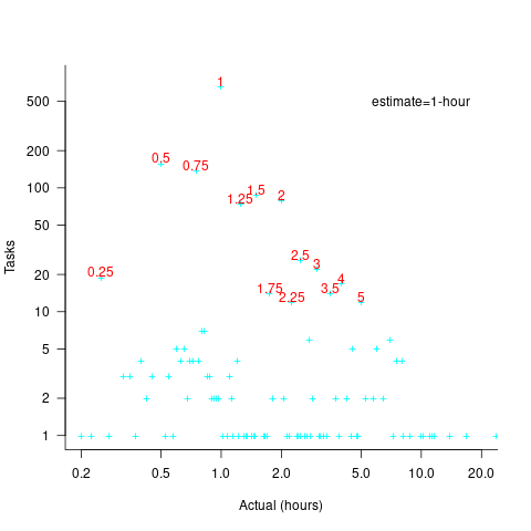
Of those 1,525 tasks estimated to take 1-hour, 44% had a reported completion time of 1-hour, 26% took less than 1-hour and 30% took more than 1-hour. The mean is 1.6 hours and the standard deviation 7.1. The spikiness of the distribution of actual times rules out analytical statistical analysis of the distribution.
If a large task is broken down into, say, smaller tasks, all estimated to take the same amount of time  , what is the distribution of actual times for the large task?
In the case of just two possible actual times to complete each smaller task, some percentage,  , of tasks are completed in actual time
  , and some percentage,
  , completed in actual time
  (with
(with  ). The probability distribution of the large task time,
 ") , for the two actual times case is:
, for the two actual times case is:
=(matrix{2}{1}{N k})(1-p_{t1})^k {p_{t1}}^{N-k}=(matrix{2}{1}{N k}){p_{t2}}^k (1-p_{t2})^{N-k}")
where:  , and
, and  .
.
The right-most equation is the probability distribution of the Binomial distribution, ") . The possible completion times for the large task start at
. The possible completion times for the large task start at  , followed by time increments of .
When there are three possible actual completion times for each smaller task, the calculation is complicated, and become more complicated with each new possible completion time.
A practical approach is to use Monte Carlo simulation. This involves simulating lots of large tasks containing smaller tasks. A sample of tasks is randomly drawn from the known 1,525 task actual times, and these actual times added to give one possible completion time. Running this process, say, 10,000 times produces what is known as the empirical distribution for the large task completion time.
The plot below shows the empirical distribution  smaller 1-hour tasks. The blue/green points show two peaks, the higher peak is a consequence of the use of round numbers, and the lower peak a consequence of the many non-round numbers. If the total times are rounded to 15 minute times, red points, a smoother distribution with a single peak emerges (code+data):

When a large task involves smaller tasks estimated to take a variety of times, the empirical distribution of the actual time for each estimated time can be combined to give an empirical distribution of the large task (see sum_prob_distrib).
Provided enough information on task completion times is available, this technique works does what it says on the tin.
Modelling time to next reported fault
After the arrival of a fault report for a program, what is the expected elapsed time until the next fault report arrives (assuming that the report relates to a coding mistake and is not a request for enhancement or something the user did wrong, and the number of active users remains the same and the program is not changed)? Here, elapsed time is a proxy for amount of program usage.
Measurements (here and here) show a consistent pattern in the elapsed time of duplicate reports of individual faults. Plotting the time elapsed between the first report and the n’th report of the same fault in the order they were reported produces an exponential line (there are often changes in the slope of this line). For example, the plot below shows 10 unique faults (different colors), the number of days between the first report and all subsequent reports of the same fault (plus character); note the log scale y-axis (discussed in this post; code+data):
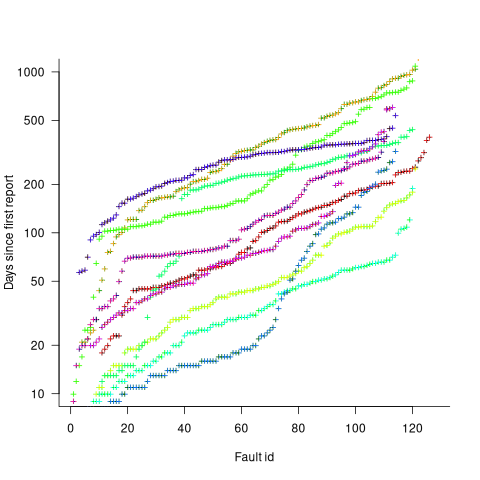
The first person to report a fault may experience the same fault many times. However, they only get to submit one report. Also, some people may experience the fault and not submit a report.
If the first reporter had not submitted a report, then the time of first report would be later. Also, the time of first report could have been earlier, had somebody experienced it earlier and chosen to submit a report.
The subpopulation of users who both experience a fault and report it, decreases over time. An influx of new users is likely to cause a jump in the rate of submission of reports for previously reported faults.
It is possible to use the information on known reported faults to build a probability model for the elapsed time between the last reported known fault and the next reported known fault (time to next reported unknown fault is covered at the end of this post).
The arrival of reports for each distinct fault can be modelled as a Poisson process. The time between events in a Poisson process with rate  has an exponential distribution, with mean
  . The distribution of a sum of multiple Poisson processes is itself a Poisson process whose rate is the sum of the individual rates. The other key point is that this process is memoryless. That is, the elapsed time of any report has no impact on the elapsed time of any other report.
If there are  different faults whose fitted report time exponents are:
  ,
,  …
…  , then summing the Poisson rates,
  , gives the mean
  , for a probability model of the estimated time to next any-known fault report.
To summarise. Given enough duplicate reports for each fault, it’s possible to build a probability model for the time to next known fault.
In practice, people are often most interested in the time to the first report of a previous unreported fault.
tl;dr Modelling time to next previously unreported fault has an analytic solution that depends on variables whose values have to be approximately approximated.
The method used to build a probability model of reports of known fault can be used extended to build a probability model of first reports of currently unknown faults. To build this model, good enough values for the following quantities are needed:
- the number of unknown faults,
 , remaining in the program. I have some ideas about estimating the number of unknown faults, , and will discuss them in another post,
 - the time,
 , needed to have received at least one report for each of the unknown faults. In practice, this is the lifetime of the program, and there is data on software half-life. However, all coding mistakes could trigger a fault report, but not all coding mistakes will have done so during a program’s lifetime. This is a complication that needs some thought,
 - the values of
 ,
,  …
…  for each of the unknown faults. There is some data suggesting that these values are drawn from an exponential distribution, or something close to one. Also, an equation can be fitted to the values of the known faults. The analysis below assumes that the
  for each unknown fault that might be reported is randomly drawn from an exponential distribution whose mean is .
This rate will be affected by program usage (i.e., number of users and the activities they perform), and source code characteristics such as the number of executions paths that are dependent on rarely true conditions.
Putting it all together, the following is the question I asked various LLMs (which uses , rather than ):
There are independent processes. Each process,  , transmits a signal, and the number of signals transmitted in a fixed time interval, , has a Poisson distribution with mean
  for
for  . The values are randomly drawn from the same exponential distribution. What is the cumulative distribution for the time between the successive first signals from the processes.
The cumulative distribution gives the probability that an event has occurred within a given amount of time, in this case the time since the last fault report.
The ChatGPT 5.2 Thinking response (Grok Thinking gives the same formula, but no chain of thought): The probability that the  unknown fault is reported within time
  of the previous report of an unknown fault,
 ") , is given by the following rather involved formula:
, is given by the following rather involved formula:
=1-(a/{a+t})^{N-k}{}_{2}F_1(N-k, k; N+1; t/{a+t})")
where: is the initial number of faults that have not been reported,  , and
, and  is the hypergeometric function.
The important points to note are: the value  decreases as more unknown faults are reported, and the dominant contribution of the value .
Deepseek’s response also makes complicated use of the same variables, and the analysis is very similar before making some simplifications that don’t look right (text of response). Kimi’s response is usually very good, but for this question failed to handle the consequences of .
Almost all published papers on fault prediction ignore the impact of number of users on reported faults, and that report time for each distinct fault has a distinct distribution, i.e., their analysis is not connected to reality.
Recent Comments