Archive
Early research on economies of scale for computer systems
Before microprocessor cost/performance wiped out (in the early 1990s) other cpu platforms (e.g., mainframes and minis), people argued that computer hardware benefited from economies of scale.
The claimed benefit was more bang for the buck, i.e., more compute for less money.
Checking this claim requires treating pre-microprocessor computer systems and the later microprocessor-based systems as two separate cases, because many of the factors driving costs and performance are very different.
Today’s large microprocessor-based computer systems achieve economies of scale through discounts from bulk purchases and spreading fixed costs across multiple systems. The data is available, and the economic analysis is straight forward.
A lack of reliable data on the costs of designing/building pre-microprocessor computer systems rules out an economic analysis of cost/performance from first principles. The data that was/is available is the cost of computer systems and some indicators of performance (such as instruction timings or benchmarks).
Now, the observed fact that the cost of compute was decreasing over time is unrelated to the claim that the cost of compute decreases as the size of the computer increases.
Assuming a power law relationship between computer cost,  , and size,
  , at a point in time, we have:
  , where
  is some constant. Economies of scale occur when:
In his detailed cost/performance analysis of computers between 1944-1967, Kenneth Knight treated computers launched in the same year as effectively occurring at the same time. He also built a single model, with year included as an explanatory variable, which means the fitted rate of decrease is the same over all years (rather than varying between years).
The plot below uses Knight’s 1953-1961 data, and shows operations per second against seconds per dollar (a confusing combination, but what Knight used), with fitted regression lines for three years using Knight’s model (code and data)
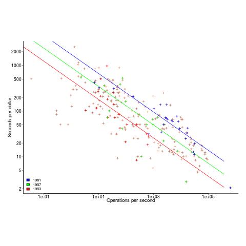
The fitted exponent for this form of x/y axis maps to a value which has , i.e., there are economies of scale.
It so happens that the value of the Knight’s fitted exponent is close to that proposed in a 1953 paper (“High speed arithmetic: The digital computer as a research tool”, no online copy):
It used to cost one cent to do a multiplication on a desk calculator; now it is more like four cents; but with these big machines we can do a million in an hour for $400, and that means twenty-five multiplications for a cent! I believe that there is a fundamental rule, which I modestly call Grosch's law, giving added economy only as the square root of the increase in speed-that is, to do a calculation ten times as cheaply you must do it one hundred times as fast. |
which did indeed become widely known as Grosch’s law.
Having been given a lucky kick-start by Knight (fitted individually, years are not close to Grosch’s law), checking for agreement with Grosch’s law became a focus for later studies. While various papers highlighted problems with the later data analysis (e.g., the regression techniques and sample noise producing mathematical artifacts), Grosch’s law ceased being a thing because mainframes/minicomputers ceased being a thing.
Did mainframe/mincomputers have economies of scale in the years after Knight’s data? It’s difficult to tell, the publicly available data is too sparse to support reliable analysis.
ISO C++ committee has a new chief sheep herder
The ISO C++ Standards committee, WG21, has a new convenor, Guy Davidson, or rather they will have when the term of the current convenor, Herb Sutter, expires at the end of this year.
Apart from the few people directly involved, this appointment does not matter to anybody (sorry Guy). The WG21 juggernaut will continue on its hedonistic way, irrespective of who is currently the chief sheep herder.
Before discussing the evolution of language standards, a brief summary of the unusual points around this appointment:
- More than one person volunteered for the job (several in the US, who selected Jeff Garland, and one in the UK; everyone agreed that both were capable candidates). The announcement by a programming language convenor that they are not standing again when their 3-year term expires more commonly kicks off discrete discussions about whose arm can be twisted to take on the role. It’s a thankless task that consumes time and money (to attend extra meetings). Also, the convenor has to be neutral, which circumscribes being involved in technical discussion.
Sometimes an outsider pops up, ruffles a few feathers and then disappears (from the Standards’ world).
- One of the SC22 (the ISO committee responsible for programming languages) convenor selection rules says (see Resolution 14-04): “When a WG Convenorship becomes vacant, … and multiple NBs have each nominated a candidate, the Convenorship shall be assigned to the candidate whose NB currently has the fewest SC 22 Convenors.” Currently, the US holds multiple convenorships and the UK holds none, so the UK nominee is appointed.
As often happens, people like diversity rules until they lose out. The US submitted a selection procedural change to SC22, and asked that it take effect before the selection of a new WG21 convenor. The overwhelming consensus at the SC22 plenary last Monday was not to change the rules while an election was in progress. An ad-hoc committee was set up to consider changes to the current rules.
End of the news and back to regular postings.
Standards committees for programming languages are now a vestige from a bygone era. The original purpose of standards was to reduce costs (the UK focused on savings achieved through repeated use of standardized items and the US focused on reduced training costs) by having companies manufacture products that conformed to a single specification.
There were once a multitude of implementations for the commercially important languages, each supporting slightly different dialects (the differences were sometimes not so slight). Language standards provided a base specification for developers interested in portable code to keep within, and that vendors could be pressured to support.
The spread of Open source compilers significantly reduced the need for companies to invest in maintaining their own compiler (there might be strategic reasons for companies selling hardware or operating systems to continue to invest in their own compiler), and reduced the likelihood that customers of commercial compiler companies would continue to pay for updates (effectively driving most compiler companies out of business).
Language standards are redundant in a monoculture, i.e., where only one compiler per language is widely used. For some years now, there have been a handful of actively maintained compilers for the widely used languages.
These days, conformance to a language standard is measured by the ability of an implementation to compile and execute the Open source software available in the various ecosystems.
As has often been observed, committees find work to keep themselves busy, and I have seen announcements for new ISO committees that look like they were created because somebody saw a CV padding opportunity.
I continue to think that the C++ committee has become a playground for bored consultants looking for a creative outlet.
WG21 meeting attendance continues to grow, now attracting 200+ attendees (Grok undercounts, e.g., 140 vs 215, and ChatGPT 5 is completely out of its depth). This is an order of magnitude greater than the C committee, WG14, and in a few years could be two orders of magnitude greater than the other SC22 languages.
The two major C/C++ compiler vendors (i.e., gcc and llvm) could simply go their own way, with regard to new language features. However, I imagine that “supporting the latest version of the language standard” is a great rationale to use when asking for funding.
How large can WG21 become before it collapses under the weight of members and the papers they write?
The POSIX standard, WG15, meetings often had 200-300 attendees in the late 1980s/early 1990s. But the POSIX committee stuck to its goal of specifying existing practice, and so has faded away.
Guy strikes me as an efficient administrator. Which is probably bad news, in the sense that this could enable WG21 to grow a lot larger. What ever happens, it will be interesting to watch.
How has the price of a computer changed over time?
We are told that computers are now orders of magnitude cheaper than they once were. Computers have changed an awful lot over the last 70 years; how is the functionality supported by different computers normalised such that the price of computers from long ago can be compared with today’s computers?
One approach is to narrow the question down to calculating the cost of performing some basic operation, e.g., numerical calculation or sorting a list of values. Nordhaus’s famous paper: Two Centuries of Productivity Growth in Computing uses this approach.
The primary advantage of the cost-of-operation approach is that it can be made to work across the complete range of computing platforms. The major disadvantage of this approach is that it focuses on the performance of the cpu/memory, ignoring the ability to store large amounts of data and perform I/O (which is most of the cost of some computer systems).
The US consumer price index (CPI) uses Hedonic regression to adjust the average price of a product family whose quality changes over time (the CPI is used to track inflation, and so every price needs to be for a product identical to the exemplar chosen at some start date). Hedonic pricing models are also used to understand how specific features within a product category (e.g., housing, automobiles, or electronics) contribute to the price. The term hedonic is derived from hedonism, and was first used in a 1939 paper analysing the price/quality of automobiles.
The 1979 paper “Hedonic Prices and the Structure of the Digital Computer Industry” by R. Michaels (cannot find a downloadable copy) appears to have kick-started the computer/hedonic research rabbit hole (the 1969 book “The Economics of Computers” by W. F. Sharpe covers computer costings in detail). Hedonic regression estimates the value of a product by braking it down into its major components which are used as the explanatory variables in a regression model that predicts the product price on given dates, e.g., for mainframe computers: price, cpu speed, amount of memory, number/size of hard disks, number of tape drives and card readers.
While mainframes and microcomputers share some characteristics (e.g., cpu, memory, and discs), they address different markets with very different requirements (e.g., mission-critical requires high reliability and tape backups). Different Hedonic regression models need to be fitted for each.
Gathering a representative sample of information on all the major components of a product, preferably for each year, is a lot of work. Many papers make use of information from proprietary databases. A lot of historical information is now available in scanned trade publications, but LLMs are not yet good enough to reliably extract detailed information from scanned documents (e.g., they sometimes ignore information, rather than hallucinating). I am waiting for the error rate to decrease.
The analysis in the book chapter Computer Processors and Peripherals by R. J. Gordon spends a lot of time dealing with the issues around potentially inconsistent data sources. The final price index (table 6.7) shows that the normalised price of mainframes decreased by a factor of 922 between 1951 and 1983 (23% per year, for 33 years). That is, the equivalent 1951 mainframe purchased in 1983 would have been cheaper by a factor of 922. In practice, prices did not decrease by a factor of 922, rather some combination of price/quality of the average mainframe changed by this factor (where quality is some combination of faster cpus, more memory and other factors). For an analysis of computer related products see the book “Price Measurements and Their Uses” by Foss, Manser, and Young.
The price of microcomputers (or computers as we call them today, as there is little public perception of any other type of computer) has decreased, but by how much (in the Hedonic sense)?
The first Hedonic analysis of microcomputers was Cohen’s 1988 Master’s thesis, for personal computers between 1976 and 1987. I think Cohen is pushing product family boundaries to treat the 8-bit computers introduced before the IBM PC in August 1981 (which did not include a hard disk until 1983, and did not really become a 16-bit computer until the IBM AT in 1987) as being comparable with later microcomputers. Cohen’s analysis found positive/negative swings in the adjusted prices of the microcomputers.
The paper Price and quality of desktop and mobile personal computers: A quarter-century historical overview by Berndt, Dulberger and Rappaport claim that there was an average annual 27% decline in microcomputer prices between 1976 and 1999. Again, my comments on pre-1987 microcomputers applies. A later paper (appendix table 1) shows average actual prices increasing until 1991 and decreasing thereafter, with the averages of cpu frequency, memory capacity and hard disk size continually increasing. There was little difference in the prices at the start(1976)/end(2002) of the period analysed, but a huge difference in the quality characteristics. While writing my Evidence-based software engineering book, I emailed Berndt for the data, which a co-author kindly made available. Unfortunately, I found that much of the data was confidential (the name of a company that sold computer sales data appeared in the files), and could not be publicly shared 🙁
Hedonic analysis of computers appears to have become unfashionable around the start of 2000. More recent papers analyse products such as mobile phones and cloud services. Please leave a comment if you know of any recent hedonic analysis of computer prices.
The only detailed microcomputer price data I know of consists of 6,259 detailed prices collected by Stengos, and Zacharias over 35 months, starting in January 1993, from the adverts in PC Magazine.
Creating a global Standard requires being politically neutral
Governments actively promote Standards because following them saves their citizens time and money. The UK and US have contrasting rationales, with the UK focusing on savings achieved through repeated use of standardized items and the US focusing on the repeated use of skills people acquired through using a standardized item (i.e., reduced training costs).
Manufacturers wanting to export products want to be able to ship identical products all over the world, i.e., not have to make costly changes for different national markets. To be able to do this, they need the rest of the world to have a Standard way of doing things. The once dominant military and industrial status of Great Britain, and now the US, motivated them to create and encourage other countries to follow the Standards they created.
These days, most programming language Standards work is done by people employed by US companies attending an international committee, SC22, with (currently) 28 countries paying to be P (participating) members and 21 countries as O (observing) members (most countries don’t appear to have any active involvement in language standards). The reason for the dominance of US companies is that few non-US companies are willing to fund staff to do Standard’s work. For a few languages SC22 essentially rubber stamps documents produced elsewhere, e.g., most of the Cobol work used to be done by a US committee and ECMAScript (aka JavaScript) work is done in a European committee mostly attended by US companies.
Other countries sometimes get to dominate the creation of a language Standard, e.g., the UK led the Pascal Standard work. At the last SC22 meeting, a person from the US lamented that Europe was set to become the dominant driver of the Ada Standard. I resisted the urge to cheer: Make Europe Great Again.
Getting an international Standard adopted throughout the world requires that ISO be politically neutral and accept any sovereign country as a member (provided they pay the membership fees). For instance, North Korea is a member of ISO.
The only politics I have previously seen in programming language standard meetings has involved company rivalry, not geopolitical rivalry. A recent request for comment from SC2 (the ISO committee responsible for coded character sets; readers are more likely to be familiar with Unicode, essentially the same information published by a non-profit consortium based in California) looks like geopolitics, in the sense of geopolitical virtue signalling.
The document is: Request for SC2 member comments on proposal to encode “Ruble sign with double vertical stem”. What does the character “Ruble sign with double vertical stem” look like? To quote the document: “The proposed character is a text element that cannot be represented by any existing character or character sequence.” Readers will have to imagine Russia’s Ruble currency symbol, ₽, with two vertical stems (I assume these stems are short antennae like lines).
What is the geopolitical connection? Readers will be aware of Russia’s invasion of Ukraine, but may not be aware of Russia’s involvement in Transnistria (quoting Wikipedia, “… a landlocked breakaway state internationally recognized as part of Moldova.”). Since 1994, the proposed character has been used as the Transnistria currency symbol.
The request for comment includes a “Non-technical considerations” section summarises various controversy points, and finishes with: “We are not aware of any non-technical criteria having been used by SC2 or WG2 in the past that could be applied to disqualify this character. We are also concerned that adopting a criterion that allows for opposing a character because of association with politically or socially defined user communities could be problematic.”
The proposed character is not included in ISO 4217 (which defines numeric codes for the representation of currencies). However, SC22 does not require that a character used to represent a currency be included in ISO 4217. Previously, SC22 has accepted currency characters that are not in ISO 4217.
Is this a one-off objection, or does it mark the start of a stream of requests to remove one or more politically incorrect characters from ISO 10646/Unicode?
A lot of people put a lot of effort into creating a unified Standard for all the characters created by the World’s people. I hope the destructive nature of virtue signalling does not take hold in programming language Standard ecosystem.
Student projects for 2024/2025
It will soon be that time of year when university students are looking for an interesting idea for a project. On an irregular basis, I post some ideas for thesis projects (here and here); primarily for students studying computing. In a change of direction, this post suggests software related ideas for business student projects.
Two idea areas require data analysis skills, one requires people skills, and one an interest in theory.
More suggestions welcome in the comments.
Career paths in software
Organizations employ people to work on software systems. What is the career path of people who work on software systems? Question include: how long people stay in a particular job or company, and salary changes over time (the only data I know of investigates the career paths of 500 people working in IT).
Governments are interested in employment, and they collect and publish data at various levels of granularity. The US Bureau of Labor Statistics contains a vast amount of information, but finding the bits of interest can require a lot of work.
In the US, government employee salary is public information, and various sites make this available, e.g., OpePayrolls and Transparent California. There is a Japanese Open Salaries, and various commercial companies operate an open salary policy (Buffer is perhaps the most famous).
This project requires students with some data analysis skills.
There is some data on job postings,
Computer company lifecycle
Companies are born, do business and eventually die (unless bought/merged). How do the lifecycle characteristics of computer companies differ from companies doing business in other domains? Lifecycle characteristics of interest might include profiles of age, number of employees, and profitability. What are the consequences, if any, of these differences?
Details of all UK registered companies are freely available from Companies House.
Open Corporates provides company information from across the world, but it is not free in bulk.
Some analysis of the geographical clustering of software companies in the UK.
This project requires students with some data analysis skills.
AI startup ecosystem
AI has exploded on the tech scene, and lots of people are creating startups to build services/products around LLMs. Teams are very fluid, with people moving around a lot looking for a viable service/product. Sometimes these teams form companies, and these might eventually leave stealth mode and become visible. What are the characteristics of the AI startup ecosystem within a city; questions include: how many people are working within it, their backgrounds, and the business areas are they focusing on?
This project requires students with people skills and a willingness to get out and about. Much of the current AI ecosystem is only visible to those within it. Evening meetups and workshops offer a way into this personal network. This research involves bootstrapping the data gathering by spending evenings schmoozing with founders and their new hires, and is probably only practical in major cities with a very active tech meeting scene.
An analysis of a Dutch software business network.
Theoretical analysis
Those with an interest in theory might like to analyse cost-benefit decision-making within software development. Examples of simple analysis+supporting data include:
Analysis of when refactoring becomes cost-effective, and Cost-effectiveness decision for fixing a known coding mistake, and Break even ratios for development investment decisions
Relative sizes of computer companies
How large are computer companies, compared to each other and to companies in other business areas?
Stock market valuation is a one measure of company size, another is a company’s total revenue (i.e., total amount of money brought in by a company’s operations). A company can have a huge revenue, but a low stock market valuation because it makes little profit (because it has to spend an almost equally huge amount to produce that income) and things are not expected to change.
The plot below shows the stock market valuation of IBM/Microsoft/Apple, over time, as a percentage of the valuation of tech companies on the US stock exchange (code+data on Github):
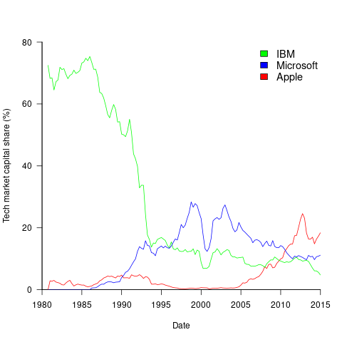
The growth of major tech companies, from the mid-1980s caused IBM’s dominant position to dramatically decline, while first Microsoft, and then Apple, grew to have more dominant market positions.
Is IBM’s decline in market valuation mirrored by a decline in its revenue?
The Fortune 500 was an annual list of the top 500 largest US companies, by total revenue (it’s now a global company list), and the lists from 1955 to 2012 are available via the Wayback Machine. Which of the 1,959 companies appearing in the top 500 lists should be classified as computer companies? Lacking a list of business classification codes for US companies, I asked Chat GPT-4 to classify these companies (responses, which include a summary of the business area). GPT-4 sometimes classified companies that were/are heavy users of computers, or suppliers of electronic components as a computer company. For instance, I consider Verizon Communications to be a communication company.
The plot below shows the ranking of those computer companies appearing within the top 100 of the Fortune 500, after removing companies not primarily in the computer business (code+data):
![]()
IBM is the uppermost blue line, ranking in the top-10 since the late-1960s. Microsoft and Apple are slowly working their way up from much lower ranks.
These contrasting plots illustrate the fact that while IBM continued to a large company by revenue, its low profitability (and major losses) and the perceived lack of a viable route to sustainable profitability resulted in it having a lower stock market valuation than computer companies with much lower revenues.
Why did organizations fund the creation of the first computers?
What were the events that drove organizations to fund the creation of the first computers?
I suspect that many readers do not appreciate how long scientific/engineering calculations took before electronic computers became available, or the huge number of clerical staff employed to process the paperwork associated with running any sizeable business.
If somebody wanted to know the logarithm of some value, or the sine/cosine of an angle, they looked up the answer in a table. Individuals owned small booklets of tables supplying some level of granularity and number of significant digits. My school boy booklet contains 60-pages of tables, all to five digits of output accuracy, with logarithm supporting four-digit input values and the sine/cosine/tangent tables having an input granularity of hundredth of a degree.
The values in these tables were calculated by human computers; with the following being among the most well known (for more details, see Calculation and Tabulation in the Nineteenth Century: Airy versus Babbage by Doron Swade, and The History of Mathematical Tables: from Sumer to Spreadsheets edited by Campbell-Kelly, Croarken, Flood, and Robson):
- In 1624 Henry Briggs published logarithms for the integer ranges 1-20,000 and 90,001-100,000 (to 14 decimal places), followed some years later by tables of sine and logarithm of sine; in 1628 Adriaan Vlacq publishing tables that filled in the missing values (to 10 decimal places). In 1783 Jurij Vega published a bug-fixed and extended version of Vlacq’s tables.
In 1827 Charles Babbage (that Babbage) published Table of Logarithms of the Natural Numbers from 1 to 10800. These tables were based on corrected versions of these tables, a rigorous nine-stage proofreading process was followed to prevent new mistakes creeping in.
Today, one person can publish A reconstruction of the tables of Briggs’ Arithmetica logarithmica (1624), with an appendix containing 300 pages of calculated values,
- between 1794 and 1799, Gaspard de Prony employed sixty to eighty computers to calculate the logarithms of the integers from 1 to 200,000 to fifteen significant digits (rounding issues sometimes required calculating 25 decimal digits; published in eighteen volumes). Around 400 man-years.
Logarithms and trigonometric functions are very widely used, creating incentives for investing in calculating and publishing tables. While it may be financially worthwhile investing in producing tables for some niche markets (e.g. Life tables for insurance companies), there is an unmet demand that will only be filled by a dramatic drop in the cost of computing simple expressions.
Babbage’s Difference engine was designed to evaluate polynomial expressions and print the results; perfect for publishing tables. While Babbage did not build a Difference engine, starting in 1837, engines based on Babbage’s design were built and sold commercially by the Swede Per Georg Scheutz.
Mechanical calculators improve accuracy and speed the process up. Vacuum tubes are invented in 1904 and become widely used to process analogue signals. World War II created an urgent demand for the results of a variety of time-consuming calculations, e.g., accurate ballistic tables, and valve computers were built. The plot below shows the cost per million operations for manual, mechanical and valve computers (code+data):
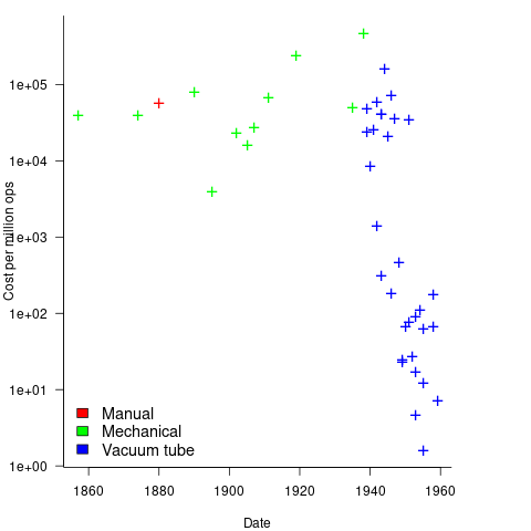
To many observers at the start of the 1950s, the market for electronic computers appeared to be organizations who needed to perform large amounts of scientific/engineering calculation.
Most businesses perform simple calculations on many unrelated values, e.g., banks have to credit/debit the appropriate account when money is deposited/withdrawn. There is no benefit in having a machine that can perform hundreds of calculations per second unless it can be fed data fast enough to keep it busy.
It so happened that, at the start of the 1950s, the US banking system was facing a crisis, the growth in the number of cheques being written meant that it would soon take longer than one day to process all the cheques that arrived in one day. In 1950 Bank of America managed 4.6 million checking accounts, and were opening 23,000 new account per month. Bank of America was then the largest bank in the world, and had a keen interest in continued growth. They funded the development of a bespoke computer system for processing cheques, the ERMA Banking system, which went live in 1959. The plot below shows the number of cheques processed per year by US banks (code+data):
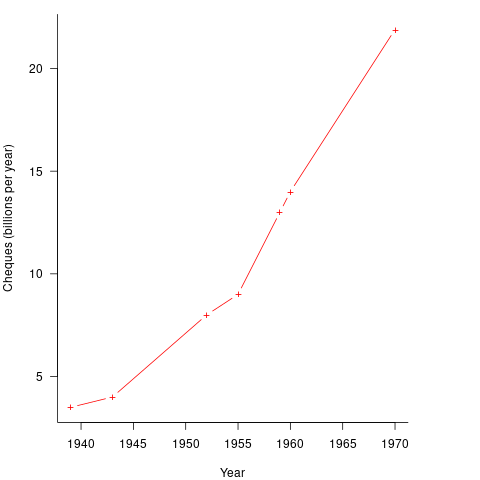
The ERMA system included electronic storage for holding account details, and data entry was speeded up by encoding account details on a magnetic strip included within every cheque.
Businesses are very interested in an integrated combination of input devices plus electronic storage plus compute. There are more commerce oriented businesses than scientific/engineering businesses, and commercial businesses usually have a lot more money to spend, i.e., the real money to be made by selling computers was the business data processing market.
The plot below shows the decreasing cost of hard disc storage (blue, right axis), along with the decreasing computing cost of valve based computers (red, left axis; code+data):
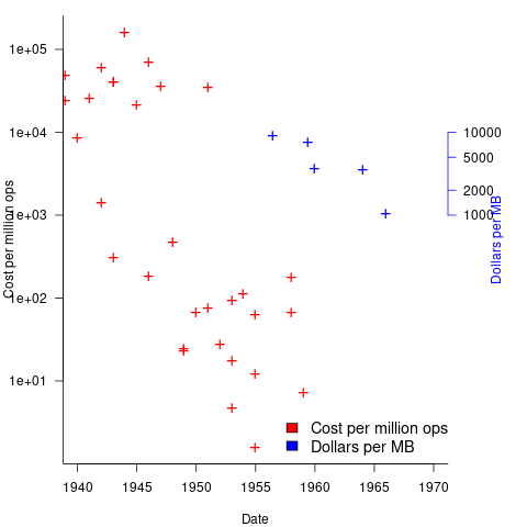
There was a larger business demand to be able to store information electronically, and the hard disc was invented by IBM, roughly 15 years after the first electronic computers.
The very different application demands of data processing and scientific/engineering are reflected in the features supported by the two languages designed in the 1950s, and widely used for the rest of the century: Cobol and Fortran.
Data processing involves simple operations on large quantities of data stored in a potentially huge number of different combinations (the myriad of mechanical point-of-sale terminals stored data in a myriad of different formats, which evolved over time, and the demand for backward compatibility created spaghetti data well before spaghetti code existed). Cobol has extensive functionality supporting the layout and format of input and output data, and simplistic coding constructs.
Scientific/engineering code involves complex calculations on some amount of input. Fortran has extensive functionality supporting program control flow, and relatively basic support for data input/output.
A third major application domain is real-time processing, such as SAGE. However, data on this domain is very hard to find, so it is not discussed.
Analysis of when refactoring becomes cost-effective
In a cost/benefit analysis of deciding when to refactor code, which variables are needed to calculate a good enough result?
This analysis compares the excess time-code of future work against the time-cost of refactoring the code. Refactoring is cost-effective when the reduction in future work time is less than the time spent refactoring. The analysis finds a relationship between work/refactoring time-costs and number of future coding sessions.
Linear, or supra-linear case
Let’s assume that the time needed to write new code grows at a linear, or supra-linear rate, as the amount of code increases ( ):
):

where:  is the base time for writing new code on a freshly refactored code base,
  is the number of lines of code that have been written since the last refactoring, and
  and
and  are constants to be decided.
The total time spent writing code over  sessions is:
^x}")
If the same number of new lines is added in every coding session,  , and is an integer constant, then the sum has a known closed form, e.g.:
x=1, ^1}={n(n+1)}/2L_s") ; x=2,
; x=2, ^2}={n(n+1)(2n+1)}/6{L_s}^2")
Let’s assume that the time taken to refactor the code written after sessions is:
^y")
where:  and
and  are constants to be decided.
The reason for refactoring is to reduce the time-cost of subsequent work; if there are no subsequent coding sessions, there is no economic reason to refactor the code. If we assume that after refactoring, the time taken to write new code is reduced to the base cost, , and that we believe that coding will continue at the same rate for at least another  sessions, then refactoring existing code after sessions is cost-effective when:
^y < k_1sum{i=n+1}{n+f}{(iL_s)^x}")
assuming that is much smaller than , setting  , and rearranging we get:

after rearranging we obtain a lower limit on the number of future coding sessions, , that must be completed for refactoring to be cost-effective after session ::

It is expected that  ; the contribution of code size, at the end of every session, in the calculation of and
  is equal (i.e.,
 ^y") ), and the overhead of adding new code is very unlikely to be less than refactoring all the newly written code.
), and the overhead of adding new code is very unlikely to be less than refactoring all the newly written code.
With  ,
,  must be close to zero; otherwise, the likely relatively large value of (e.g., 100+) would produce surprisingly high values of .
Sublinear case
What if the time overhead of writing new code grows at a sublinear rate, as the amount of code increases?
Various attributes have been found to strongly correlate with the  of lines of code. In this case, the expressions for and become:

")
and the cost/benefit relationship becomes:
 < k_1sum{i=n+1}{n+f}{log(iL_s)}")
applying Stirling’s approximation and simplifying (see Exact equations for sums at end of post for details) we get:
 < k_1(f(log(n+f)-1)+f log{L_s})")
+log{L_s}-1} < f")
applying the series expansion (for  ):
):  , we get
 < f")
Discussion
What does this analysis of the cost/benefit relationship show that was not obvious (i.e., the relationship  is obviously true)?
What the analysis shows is that when real-world values are plugged into the full equations, all but two factors have a relatively small impact on the result.
A factor not included in the analysis is that source code has a half-life (i.e., code is deleted during development), and the amount of code existing after sessions is likely to be less than the  used in the analysis (see Agile analysis).
As a project nears completion, the likelihood of there being more coding sessions decreases; there is also the every present possibility that the project is shutdown.
The values of and encode information on the skill of the developer, the difficulty of writing code in the application domain, and other factors.
Exact equations for sums
The equations for the exact sums, for  , are:
")
+1)")
(2n(n+1)+2fn+f+f^2)")
-zeta(-0.5, f+n+1)") , where
, where  is the Hurwitz zeta function.
Sum of a log series: !}/{n!}}+f log{L_s}")
using Stirling’s approximation we get
!)}-log(n!) approx (n+f-0.5)log(n+f)-(n+f)-((n-0.5)log n-n)")
simplifying
!)}-log(n!) approx (n-0.5)log(1+f/n)+f log(n+f)-f")
and assuming that is much smaller than gives
!)}-log(n!) approx f(log(n+f)-1)")
Update
The analysis above assumes that the time contribution of the base rate, , is independent of the changes,  . The following analysis combines these two contributions into a single rate:
L)^b}")
where: ,  , , and are positive constants, with
  , and
, and  .
.
The following is a very good approximation to this sum (thanks to Grok 4.1 beta; chat script):
L})")
where: L")
Unneeded requirements implemented in Waterfall & Agile
Software does not wear out, but the world in which it runs evolves. Time and money is lost when, after implementing a feature in software, customer feedback is that the feature is not needed.
How do Waterfall and Agile implementation processes compare in the number of unneeded feature/requirements that they implement?
In a Waterfall process, a list of requirements is created and then implemented. The identity of ‘dead’ requirements is not known until customers start using the software, which is not until it is released at the end of development.
In an Agile process, a list of requirements is used to create a Minimal Viable Product, which is released to customers. An iterative development processes, driven by customer feedback, implements requirements, and makes frequent releases to customers, which reduces the likelihood of implementing known to be ‘dead’ requirements. Previously implemented requirements may be discovered to have become ‘dead’.
An analysis of the number of ‘dead’ requirements implemented by the two approaches appears at the end of this post.
The plot below shows the number of ‘dead’ requirements implemented in a project lasting a given number of working days (blue/red) and the difference between them (green), assuming that one requirement is implemented per working day, with the discovery after 100 working days that a given fraction of implemented requirements are not needed, and the number of requirements in the MVP is assumed to be small (fractions 0.5, 0.1, and 0.05 shown; code):
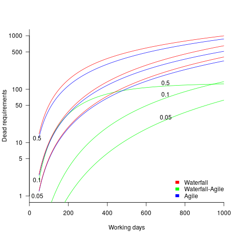
The values calculated using one requirement implemented per day scales linearly with requirements implemented per day.
By implementing fewer ‘dead’ requirements, an Agile project will finish earlier (assuming it only implements all the needed requirements of a Waterfall approach, and some subset of the ‘dead’ requirements). However, unless a project is long-running, or has a high requirements’ ‘death’ rate, the difference may not be compelling.
I’m not aware of any data on rate of discovery of ‘dead’ implemented requirements (there is some on rate of discovery of new requirements); as always, pointers to data most welcome.
The Waterfall projects I am familiar with, plus those where data is available, include some amount of requirement discovery during implementation. This has the potential to reduce the number of ‘dead’ implemented requirements, but who knows by how much.
As the size of Minimal Viable Product increases to become a significant fraction of the final software system, the number of fraction of ‘dead’ requirements will approach that of the Waterfall approach.
There are other factors that favor either Waterfall or Agile, which are left to be discussed in future posts.
The following is an analysis of Waterfall/Agile requirements’ implementation.
Define:
 is the fraction of requirements per day that remain relevant to customers. This value is likely to be very close to one, e.g.,
  .
.
 requirements implemented per working day.
Waterfall
The implementation of  requirements takes
  days, and the number of implemented ‘dead’ requirements is (assuming that the no ‘dead’ requirements were present at the end of the requirements gathering phase):
")
As  effectively all implemented requirements are ‘dead’.
Agile
The number of implemented ‘live’ requirements on day is given by:

with the initial condition that the number of implemented requirements at the start of the first day of iterative development is the number of requirements implemented in the Minimum Viable Product, i.e.,  .
.
Solving this difference equation gives the number of ‘live’ requirements on day :
+F_{live}}")
as  ,
,  approaches to its maximum value of
Subtracting the number of ‘live’ requirements from the total number of requirements implemented gives:

or
+n*R_{done}(1-1/{n(1-F_{live})+F_{live}})")
or
+n*R_{done}{n-1}/{n+F_{live}/(1-F_{live})}")
as effectively all implemented requirements are ‘dead’, because the number of ‘live’ requirements cannot exceed a known maximum.
Update
The paper A software evolution experiment found that in a waterfall project, 40% of modules in the delivered system were not required.
Optimal sizing of a product backlog
Developers working on the implementation of a software system will have a list of work that needs to be done, a to-do list, known as the product backlog in Agile.
The Agile development process differs from the Waterfall process in that the list of work items is intentionally incomplete when coding starts (discovery of new work items is an integral part of the Agile process). In a Waterfall process, it is intended that all work items are known before coding starts (as work progresses, new items are invariably discovered).
Complaints are sometimes expressed about the size of a team’s backlog, measured in number of items waiting to be implemented. Are these complaints just grumblings about the amount of work outstanding, or is there an economic cost that increases with the size of the backlog?
If the number of items in the backlog is too low, developers may be left twiddling their expensive thumbs because they have run out of work items to implement.
A parallel is sometimes drawn between items waiting to be implemented in a product backlog and hardware items in a manufacturer’s store waiting to be checked-out for the production line. Hardware occupies space on a shelf, a cost in that the manufacturer has to pay for the building to hold it; another cost is the interest on the money spent to purchase the items sitting in the store.
For over 100 years, people have been analyzing the problem of the optimum number of stock items to order, and at what stock level to place an order. The economic order quantity gives the optimum number of items to reorder,  (the derivation assumes that the average quantity in stock is
  ), it is given by:
 , where
  is the quantity consumed per year,
  is the fixed cost per order (e.g., cost of ordering, shipping and handling; not the actual cost of the goods),
  is the annual holding cost per item.
What is the likely range of these values for software?
- is around 1,000 per year for a team of ten’ish people working on multiple (related) projects; based on one dataset,
- is the cost associated with the time taken to gather the requirements, i.e., the items to add to the backlog. If we assume that the time taken to gather an item is less than the time taken to implement it (the estimated time taken to implement varies from hours to days), then the average should be less than an hour or two,
- : While the cost of a post-it note on a board, or an entry in an online issue tracking system, is effectively zero, there is the time cost of deciding which backlog items should be implemented next, or added to the next Sprint.
If the backlog starts with
items, and it takes  seconds to decide whether a given item should be implemented next, and is the fraction of items scanned before one is selected: the average decision time per item is:
 /2}*t") seconds. For example, if
seconds. For example, if  , pulling some numbers out of the air,
  , and
, and  , then
  , or 5.4 minutes.
The Scrum approach of selecting a subset of backlog items to completely implement in a Sprint has a much lower overhead than the one-at-a-time approach.
If we assume that  , then
  .
.
An ‘order’ for 45 work items might make sense when dealing with clients who have formal processes in place and are not able to be as proactive as an Agile developer might like, e.g., meetings have to be scheduled in advance, with minutes circulated for agreement.
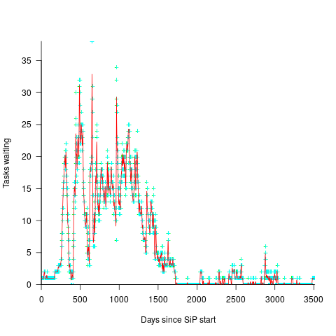
In a more informal environment, with close client contacts, work items are more likely to trickle in or appear in small batches. The SiP dataset came from such an environment. The plot below shows the number of tasks in the backlog of the SiP dataset, for each day (blue/green) and seven-day rolling average (red) (code+data):
Recent Comments