The Shape of Code

Developers working on the implementation of a software system will have a list of work that needs to be done, a to-do list, known as the product backlog in Agile.

The Agile development process differs from the Waterfall process in that the list of work items is intentionally incomplete when coding starts (discovery of new work items is an integral part of the Agile process). In a Waterfall process, it is intended that all work items are known before coding starts (as work progresses, new items are invariably discovered).

Complaints are sometimes expressed about the size of a team’s backlog, measured in number of items waiting to be implemented. Are these complaints just grumblings about the amount of work outstanding, or is there an economic cost that increases with the size of the backlog?

If the number of items in the backlog is too low, developers may be left twiddling their expensive thumbs because they have run out of work items to implement.

A parallel is sometimes drawn between items waiting to be implemented in a product backlog and hardware items in a manufacturer’s store waiting to be checked-out for the production line. Hardware occupies space on a shelf, a cost in that the manufacturer has to pay for the building to hold it; another cost is the interest on the money spent to purchase the items sitting in the store.

For over 100 years, people have been analyzing the problem of the optimum number of stock items to order, and at what stock level to place an order. The economic order quantity gives the optimum number of items to reorder, (the derivation assumes that the average quantity in stock is ), it is given by:

, where is the quantity consumed per year, is the fixed cost per order (e.g., cost of ordering, shipping and handling; not the actual cost of the goods), is the annual holding cost per item.

What is the likely range of these values for software?

• is around 1,000 per year for a team of ten’ish people working on multiple (related) projects; based on one dataset,
• is the cost associated with the time taken to gather the requirements, i.e., the items to add to the backlog. If we assume that the time taken to gather an item is less than the time taken to implement it (the estimated time taken to implement varies from hours to days), then the average should be less than an hour or two,
• : While the cost of a post-it note on a board, or an entry in an online issue tracking system, is effectively zero, there is the time cost of deciding which backlog items should be implemented next, or added to the next Sprint.

  If the backlog starts with items, and it takes seconds to decide whether a given item should be implemented next, and is the fraction of items scanned before one is selected: the average decision time per item is: seconds. For example, if , pulling some numbers out of the air, , and , then , or 5.4 minutes.

  The Scrum approach of selecting a subset of backlog items to completely implement in a Sprint has a much lower overhead than the one-at-a-time approach.

If we assume that , then .

An ‘order’ for 45 work items might make sense when dealing with clients who have formal processes in place and are not able to be as proactive as an Agile developer might like, e.g., meetings have to be scheduled in advance, with minutes circulated for agreement.

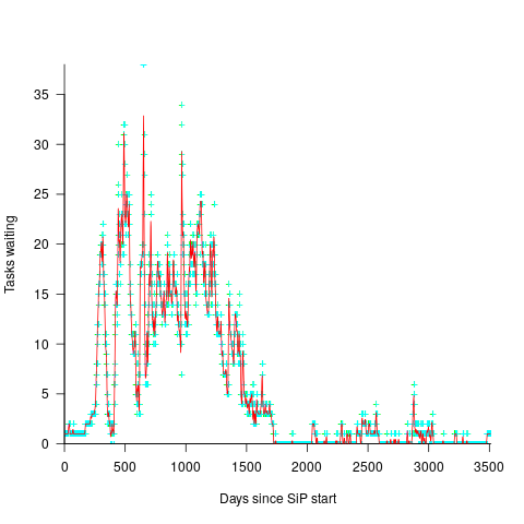
In a more informal environment, with close client contacts, work items are more likely to trickle in or appear in small batches. The SiP dataset came from such an environment. The plot below shows the number of tasks in the backlog of the SiP dataset, for each day (blue/green) and seven-day rolling average (red) (code+data):