Archive
Lifetime of coding mistakes in the Linux kernel
What is the lifetime of coding mistakes in the Linux kernel? Some coding mistakes result in fault reports (some of which are fixed), while many are removed when the source that contains them is deleted/changed during ongoing development.
After fixing the coding mistake(s) in the kernel that generated a reported fault, developer(s) log the commit that introduced the coding mistake, along with the commit that fixed it. This logging started in 2013, and I only found out about it this week. To be exact, I discovered the repo: A dataset of Linux Kernel commits created by Maes Bermejo, Gonzalez-Barahona, Gallego, and Robles.
The log contains the commit hashes for the 90,760 fixes made to the 63 mainline kernel versions from 3.12 to 6.13. The complete log of 1,233,421 commits has to be searched to extract the details, e.g., date, lines added, etc.
The kernel development process involves regular release cycles of around 80 days. Developers submit the code they want to be included in the next release, this goes through a series of reviews, with Linus making the final decision.
The following analysis is based on the coding mistakes introduced between successive kernel releases, e.g., version 3.13 coding mistakes are those introduced into the source between 4 Nov 2013 (the day after version 3.12 was released) and 19 Jan 2014 (when version 3.13 was released). Code will have been worked on, and mistakes created/fixed, before it reached the kernel, which ensures some level of maturity.
The number of people working with pre-release code is likely to be tiny, compared to the number running released kernels. Consequently, the characteristics of coding mistake lifetime is expected to be different pre/post release, if only because more users are likely to report more faults.
The plot below shows the pre-release daily mistake fixed density against days since start of work on the current release, the red line is a fitted regression line mapped to density (fitted regression is a biexponential; code and data):
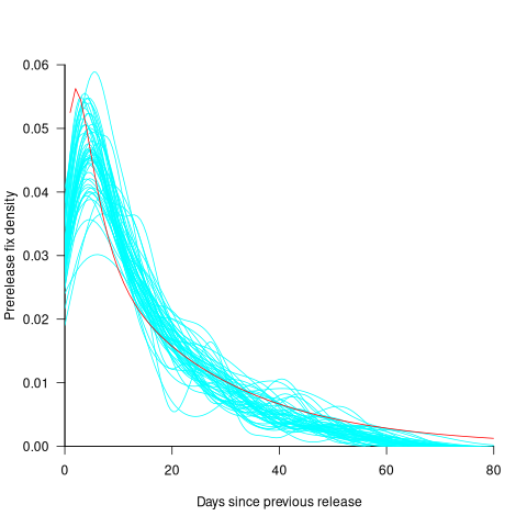
For all versions, the prior to release daily fix rate follows a consistent pattern: Most fixes occur in the first few days, with roughly an exponential decline to the release date.
The following analysis builds a broad brush model of cumulative fixes over time across 53 mainline kernel releases (the final 10 releases were not included because of their relatively short history).
The number of users of a new kernel takes time to increase as it percolates onto systems, e.g., adopted by Linux distributions and then installed by users, or installed by cloud providers. Eventually, code first included in a particular version will be running on most systems.
The post release daily fix rate is best modelled using the cumulative number of fixes, i.e., total number of fixes up to a given day since release. The models fitted below are based on dividing the post release cumulative fixes into before/after 200 days since release. The 200-day division is a round number (technically, a nearby value may provide a better fit) that supports the fitting of good quality before/after regression models. Averaged over all releases, 42% of fixes occurred within 200-days, and 58% after 200-days.
The plot below shows the cumulative number of post-release fixed faults, in red, for various kernel versions, with fitted regression lines in green and blue (grey line is at 200-days; code and data):

The equation fitted to the before 200-days fixes had the following form:
}")
where:  is a kernel version specific constant; see plot below.
The equation fitted to the after 200-days fixes had the following form:

where:  is a kernel version specific constant; see plot below.
Approximately, after release, the cumulative fix rate starts out quadratic in elapsed days, with the rate decreasing over time, until after 200-days the rate settles down to following the cube-root of days.
Comparing the number of post-release fixes across versions, there is a lot more variability in the first 200-days (i.e., the model fit to the data is sometimes very poor), relatively to after 200-days (where the model fit is consistently good).
Each kernel release has its own characteristics, parameterised by the values , and in the above equations. The plot below shows these values across versions, with red for , blue/green for , and grey line showing normalised LOC added/changed in the release (code and data):
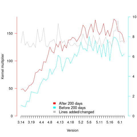
The plot clearly shows a large increase in the number of fixes between kernel version 3.14 and later versions. The before 200-days rate (blue/green) increase by a factor of seven, while the after 200-days rate increased by a factor of three.
Is this increase driven by some underlying factor in kernel development, or is it an external factor such as an increase in the number of users (more users leads to more faults reports), or the extensive post-release fuzz testing that is now common.
The number of lines of code added/changed, indicated by the grey line (shifted to fit plot axes) cannot be added to the fitted models because they exactly correlate with their respective version.
What is driving the long-term rate of fixes, i.e., cube-root of elapsed days?
Actually, what people are really want to know is what can be done to reduce the number of fixes required after release. When people ask me this, my usual reply is: “Spend more on testing”.
The probability of a coding mistake causing a fault report is decreasing: fixes reduce the number of remaining mistakes, and source added in one kernel version may be removed in a later version.
Perhaps the set of input behaviors is growing, producing the distinct conditions needed to trigger different coding mistakes, or the faults are occurring but are only reported when experienced by a small subset of users.
As always, more data is needed.
Optimal function length: an analysis of the cited data
Careful analysis is required to extract reliable conclusions from data. Sloppy analysis can lead to incorrect conclusions being drawn.
The U-shaped plots cited as evidence for an ‘optimal’ number of LOC in a function/method that minimises the number of reported faults in a function, were shown to be caused by a mathematical artifact. What patterns of behavior are present in the data cited as evidence for an optimal number of LOC?
The 2000 paper Module Size Distribution and Defect Density by Malaiya and Denton summarises the data-oriented papers cited as sources on the issue of optimal length of a function/method, in LOC.
Note that the named unit of measurement in these papers is a module. In one paper, a module is specified as being as Ada package, but these papers specify that a module is a single function, method or anything else.
In order of publication year, the papers are:
The 1984 paper Software errors and complexity: an empirical investigation by Basili, and Perricone analyses measurements from a 90K Fortran program. The relevant Faults/LOC data is contained in two tables (VII and IX). Modules are sorted in to one of five bins, based on LOC, and average number of errors per thousand line of code calculated (over all modules, and just those containing at least one error); see table below:
     Module         Errors/1k lines   Errors/1k lines
     max LOC          all modules      error modules
        50              16.0               65.0
       100              12.6               33.3
       150              12.4               24.6
       200               7.6               13.4
>200 6.4 9.7 |
One of the paper’s conclusions: “One surprising result was that module size did not account for error proneness. In fact, it was quite the contrary–the larger the module, the less error-prone it was.”
The 1985 paper Identifying error-prone software—an empirical study by Shen, Yu, Thebaut, and Paulsen analyses defect data from three products (written in Pascal, PL/S, and Assembly; there were three versions of the PL/S product) were analysed using Halstead/McCabe, plus defect density, in an attempt to identify error-prone software.
The paper includes a plot (figure 4) of defect density against LOC for one of the PL/S product releases, for 108 modules out of 253 (presumably 145 modules had no reported faults). The plot below shows defects against LOC, the original did not include axis values, and the red line is the fitted regression model  (data extracted using WebPlotDigitizer; code+data):
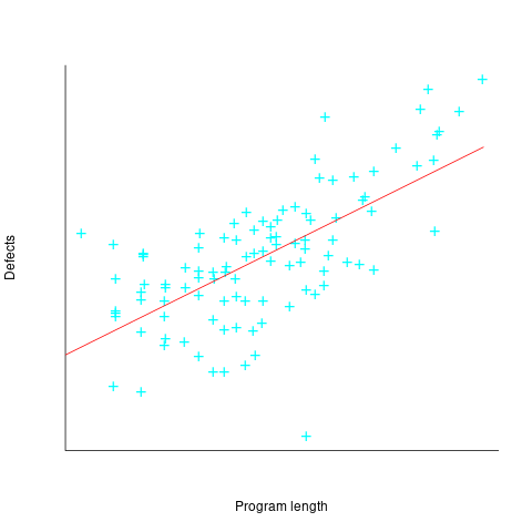
The power-law exponent is less than one, which suggests that defects per line is decreasing as module size increases, i.e., there is no optimal minimum, larger is always better. However, the analysis is incomplete because it does not include modules with zero reported defects.
The authors say: “… that there is a higher mean error rate in smaller sized modules, is consistent with that discovered by Basili and Perricone.”
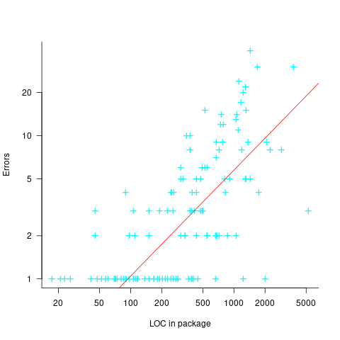
The 1990 paper Error Density and Size in Ada Software by Carol Withrow analyses error data from a 114 KLOC military communication system written in Ada; of the 362 Ada packages, 137 had at least one error. The unit of measurement is an Ada package, which like a C++ class, can contain multiple definitions of types, variables, and functions.
The paper plots errors per thousand line of code against LOC, for packages containing at least one error, i.e., 62% of packages are not included in the analysis. The 137 packages are sorted into 8-bins, based on the number of lines they contain. The 52 packages in the 159-251 LOC bin have an average of 1.8 errors per 1 KLOC, which is the lowest bin average. The author concludes: “Our study of a large Ada project shows this optimal size to be about 225 lines.”
The plot below shows errors against LOC, red line is the fitted regression model  for
for  (data extracted using WebPlotDigitizer from figure 2; code+data):
The 1993 paper An Empirical Investigation of Software Fault Distribution by Moller, and Paulish analysed four versions of a 750K product for controlling computer system utilization, written in assembler; the items measured were: DLOC (‘delta’ lines of code, DLOC, defined as “… the number of added or modified source lines of code for a version as compared to the prior version.”) and fault rate (faults per DLOC).
This paper is the first to point out that the code from multiple modules may need to be modified to fix a defect/fault/error. The following table shows the percentage of faults whose correction required changes to a given number of modules, for three releases of the product.
                   Modules
   Version  1    2    3     4     5     6
      a    78%  14%  3.4%  1.3%  0.2%  0.1%
      b    77%  18%  3.3%  1.1%  0.3%  0.4%
c 85% 12% 2.0% 0.7% 0.0% 0.0% |
Modules are binned by DLOC and various plots appear in the paper; it’s all rather convoluted. The paper summary says: “With modified code, the fault rates steadily decrease as the module size increases.”
What conclusions does the Malaiya and Denton paper draw from these papers?
They present “… a model giving influence of module size on defect density based on data that has been reported. It provides an interpretation for both declining defect density for smaller modules and gradually rising defect density for larger modules. … If small modules can be
combined into optimal sized modules without reducing cohesion significantly, than the inherent defect density may be significantly reduced.”
The conclusion I draw from these papers is that a sloppy analysis in one paper obtained a result that sounded interesting enough to get published. All the other papers find defect/error/fault rate decreasing with module size (whatever a module might be).
Low defect density implies climate code less, not more, reliable
I have just been reading a paper comparing the defect density of three climate modelling systems against software from other application domains. The defect density (total reported defects divided by thousands of lines of code) of the climate modelling software was significantly lower than everything else, leading the researchers to conclude that “… suggests that the models are of high software quality,”. I would draw the opposite conclusion, the models have low reliability (I have no idea what software quality is and avoid using the term).
I don’t disagree with Pipitone and Easterbrook numbers, just their conclusion.
There is a very simple technique for creating software that has a low defect density, don’t try too hard to look for defects. There are two reasons why I think this has happened with the climate model software:
- Three of the non-climate systems compared against were the Apache HTTP demon, the VTK visulalization toolkit and the Eclipse project. These are all widely used projects with many thousands of users, millions for Apache; this volume of usage corresponds to a huge amount of testing, and it is no wonder that so many faults have been reported. Each climate model tends to be used by one site, a tiny amount of testing, and it is not surprising that few faults have been reported.
- Climate models have a big intrinsic testing problem; what is the result of a test supposed to be? With applications such as word processors, browsers, compilers, operating systems, etc the expected behavior is known in many cases so it is possible to write test cases that check for the expected behavior. How does anybody know what the expected behavior of a climate model is? If all the climate models did was to solve the Navier-Stokes equation on a rotating sphere there would be no need for multiple models and the UK Meteorological Office’s Unified model would not have grown from 100 KLOC to 800+ KLOC over the last 15 years.
The one system having a similar defect density to the climate models that Pipitone and Easterbrook compare against is an air traffic control system developed using formal methods, exactly the kind of (expensive and time-consuming) development process that one would expect to have a low defect density.
Software is remarkably fault-tolerant and so, yes, serious fault could exist in the climate models and they would still give answers that looked about right. Based on his experience working on a meteorological model Les Hatton tells the story of a fault so serious that the answers should be completely wrong, but they were not.
If somebody wants to convince me that the software in any of these climate models really is reliable then I want to know about the test suites used to check the behavior; what coverage of the source does the suite have (a high MC/DC would be very good, but I would settle for a very high statement coverage) and how were the expected behaviors calculated.
Recent Comments