Optimal function length: an analysis of the cited data
Careful analysis is required to extract reliable conclusions from data. Sloppy analysis can lead to incorrect conclusions being drawn.
The U-shaped plots cited as evidence for an ‘optimal’ number of LOC in a function/method that minimises the number of reported faults in a function, were shown to be caused by a mathematical artifact. What patterns of behavior are present in the data cited as evidence for an optimal number of LOC?
The 2000 paper Module Size Distribution and Defect Density by Malaiya and Denton summarises the data-oriented papers cited as sources on the issue of optimal length of a function/method, in LOC.
Note that the named unit of measurement in these papers is a module. In one paper, a module is specified as being as Ada package, but these papers specify that a module is a single function, method or anything else.
In order of publication year, the papers are:
The 1984 paper Software errors and complexity: an empirical investigation by Basili, and Perricone analyses measurements from a 90K Fortran program. The relevant Faults/LOC data is contained in two tables (VII and IX). Modules are sorted in to one of five bins, based on LOC, and average number of errors per thousand line of code calculated (over all modules, and just those containing at least one error); see table below:
     Module         Errors/1k lines   Errors/1k lines
     max LOC          all modules      error modules
        50              16.0               65.0
       100              12.6               33.3
       150              12.4               24.6
       200               7.6               13.4
>200 6.4 9.7 |
One of the paper’s conclusions: “One surprising result was that module size did not account for error proneness. In fact, it was quite the contrary–the larger the module, the less error-prone it was.”
The 1985 paper Identifying error-prone software—an empirical study by Shen, Yu, Thebaut, and Paulsen analyses defect data from three products (written in Pascal, PL/S, and Assembly; there were three versions of the PL/S product) were analysed using Halstead/McCabe, plus defect density, in an attempt to identify error-prone software.
The paper includes a plot (figure 4) of defect density against LOC for one of the PL/S product releases, for 108 modules out of 253 (presumably 145 modules had no reported faults). The plot below shows defects against LOC, the original did not include axis values, and the red line is the fitted regression model  (data extracted using WebPlotDigitizer; code+data):
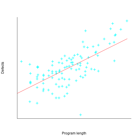
The power-law exponent is less than one, which suggests that defects per line is decreasing as module size increases, i.e., there is no optimal minimum, larger is always better. However, the analysis is incomplete because it does not include modules with zero reported defects.
The authors say: “… that there is a higher mean error rate in smaller sized modules, is consistent with that discovered by Basili and Perricone.”
The 1990 paper Error Density and Size in Ada Software by Carol Withrow analyses error data from a 114 KLOC military communication system written in Ada; of the 362 Ada packages, 137 had at least one error. The unit of measurement is an Ada package, which like a C++ class, can contain multiple definitions of types, variables, and functions.
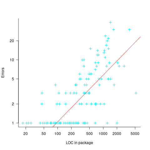
The paper plots errors per thousand line of code against LOC, for packages containing at least one error, i.e., 62% of packages are not included in the analysis. The 137 packages are sorted into 8-bins, based on the number of lines they contain. The 52 packages in the 159-251 LOC bin have an average of 1.8 errors per 1 KLOC, which is the lowest bin average. The author concludes: “Our study of a large Ada project shows this optimal size to be about 225 lines.”
The plot below shows errors against LOC, red line is the fitted regression model  for
for  (data extracted using WebPlotDigitizer from figure 2; code+data):
The 1993 paper An Empirical Investigation of Software Fault Distribution by Moller, and Paulish analysed four versions of a 750K product for controlling computer system utilization, written in assembler; the items measured were: DLOC (‘delta’ lines of code, DLOC, defined as “… the number of added or modified source lines of code for a version as compared to the prior version.”) and fault rate (faults per DLOC).
This paper is the first to point out that the code from multiple modules may need to be modified to fix a defect/fault/error. The following table shows the percentage of faults whose correction required changes to a given number of modules, for three releases of the product.
                   Modules
   Version  1    2    3     4     5     6
      a    78%  14%  3.4%  1.3%  0.2%  0.1%
      b    77%  18%  3.3%  1.1%  0.3%  0.4%
c 85% 12% 2.0% 0.7% 0.0% 0.0% |
Modules are binned by DLOC and various plots appear in the paper; it’s all rather convoluted. The paper summary says: “With modified code, the fault rates steadily decrease as the module size increases.”
What conclusions does the Malaiya and Denton paper draw from these papers?
They present “… a model giving influence of module size on defect density based on data that has been reported. It provides an interpretation for both declining defect density for smaller modules and gradually rising defect density for larger modules. … If small modules can be
combined into optimal sized modules without reducing cohesion significantly, than the inherent defect density may be significantly reduced.”
The conclusion I draw from these papers is that a sloppy analysis in one paper obtained a result that sounded interesting enough to get published. All the other papers find defect/error/fault rate decreasing with module size (whatever a module might be).
Halstead & McCabe metrics: The wisdom of the ancients
Study after study finds that the predictive power of both the Halstead metric and the McCabe cyclomatic complexity metric is no better than counting lines of code, for the characteristics of interest. Why do people continue to use and cite the Halstead and McCabe metrics?
My experience, talking to people, is that many believe these metrics have greater predictive power than lines of code. Sometimes I explain the situation, other times I move on.
Those who are aware of the facts often continue to use these metrics. Why do they do this?
Given the lack of alternative metrics that are more effective than lines of code, for the claimed uses of Halstead/McCabe, following the herd is the easy option (I regularly point this out to people, after explaining that Halstead/McCabe don’t do what is claimed on the tin). Tools are available to calculate the metrics; the manual effort is clicking buttons or running a command.
Why were the Halstead/McCabe metrics ‘successful’, in that they are the ones people cite/use today?
Both were formulated in the mid-1970s, when the discussion around measuring software started in earnest, so they had some first-mover advantage (within a few years they were both being suggested for use by US Military). Individuals promoted their ideas: Maurice Halstead was a senior professor, with colleagues and lots of graduate students, who advertised the metric via their publications; Thomas McCabe was working for the NSA when his famous paper was published, and went on to form a company working in the area of source code analysis.
The Halstead/McCabe metrics can both be calculated by processing the source one line at a time (just count decision points for McCabe, no need for the pretentious graph theory stuff). In the 1970s, computer memory was often measured in kilobytes, which made it difficult to implement complicated metrics that required keeping dependency information in memory.
Metrics based on the subroutine/function/procedure/method as the measured unit of source code had an implementation and usage advantage over metrics based on larger units of code.
In the 1990s, object-oriented programming, in the form of C++ and then Java, took off. The common view, by those caught up in the times, was that object-oriented software was so different from what went before that it needed its own metrics.
The 1991 paper: Towards a Metrics Suite for Object Oriented Design, by Chidamber and Kemerer, introduced the six CK metrics (as they become known; 1992 update). The nearest this paper comes to citing the Halstead/McCabe work is to say: “Some early work has recognized the shortcomings of existing metrics and the need for new metrics especially designed for OO.” The paper followed in the footsteps of the earlier work in not providing any evidence for the claims made (the update contains histograms of metric values from a C++ project and a Smalltalk project).
The 1996 paper: Evaluating the Impact of Object-Oriented Design on Software Quality, by Abreu and Melo, introduced the MOOD metrics (Metrics for Object-Oriented Design).
At the end of 2022 the total citation counts returned by Google Scholar were: McCabe 8,670, Halstead 4,900, CK 8,160, and MOOD 354.
The plot below shows the number of new citations returned by Google Scholar, each year, for the respective metrics papers (or book for Halstead; code+data):
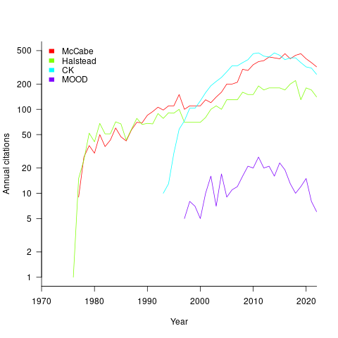
The ongoing growth in annual rate of citation probably has more to do with the growth in the number of software papers published each year, rather than these metric papers being cited by an expanding number of research fields.
Do authors tend to cite one or the other of Halstead/McCabe, or both?
Using Google Scholar’s ‘search within’ option to find the subset of papers that included a string matching the title of a paper: 46% of the Halstead citations include a citation of the McCabe paper, and 25% of the McCabe citations include a citation of the Halstead paper.
The Inciteful’s paper network (with citation counts: Halstead 1,052 and McCabe 4,970) found 657 papers citing both (62% of the Halstead total, 12% of the McCabe).
It’s not possible to make use of the OpenCitations API because it is DOI based, and the Halstead citation is a book.
Readability of anonymous inner classes and lambda expressions
The available evidence on readability is virtually non-existent, mostly consisting of a handful of meaningless experiments.
Every now and again somebody runs an experiment comparing the readability of X and Y. All being well, this produces a concrete result that can be published. I think that it would be a much more effective use of resources to run eye tracking experiments to build models of how people read code, but then I’m not on the publish or perish treadmill.
One such experimental comparison of X and Y is the paper Two N-of-1 self-trials on readability differences between anonymous inner classes (AICs) and lambda expressions (LEs) on Java code snippets by Stefan Hanenberg (who ran some experiments on the benefits of strong typing) and Nils Mehlhorn.
How might the readability of X and Y be compared (e.g., Java anonymous inner classes and lambda expressions)?
If the experimenter has the luxury of lots of subjects, then half of the subjects can be assigned to use X and half to use Y. When only a few subjects are available, perhaps as few as one, an N-of-1 experimental design can be used.
This particular study is worth discussing because it appears to be thought out and well run, as well as illustrating the issues involved in running such experiments, not because the readability of the two constructs is of particular interest. I think that developer choice of anonymous inner classes or lambda expressions is based on fashion and/or habit, and developers will claim the construct they use is the most readable one for them.
The Hanenberg and Mehlhorn study involved two experiments, using a N-of-1 design. In the first experiment task, subjects saw a snippet of code and had to count the number of parameters in either the anonymous inner class or the lambda expression (whose parameters were either untyped or typed); in the second experiment task subjects had to count the number of defined parameters that were used in the body of the anonymous inner class or lambda expression. English words were used for parameter names.
Each of the eight subjects saw the same set of randomly shuffled distinct 600 code snippets. The time taken to answer and correct/incorrect answer status were recorded. The snippets varied in the number of parameters and kind of construct; for task 1: 0-4 parameters, 3-kinds of construct, repeated 40 times, giving  distinct snippets; for task 2: 0-3 parameters used out of 3 parameters, 3-kinds of construct, repeated 50 times, giving
  distinct snippets.
The first task requires subjects to locate the definition of the construct, count the number of parameters, and report the count. The obvious model is different constructs require different amounts of time to locate, and that each parameter adds a fixed amount to the response time; there may be a small learning component.
Fitting a simple regression model shows (depending on choice of outlier bounds) that averaged over all subjects each parameter increased response time by around 80 msec, and that response was faster for lambda expressions (around 200 msec without parameter types, 90 msec if types are present); code+data. However, the variation across subjects had a standard deviation that was similar to these means.
The second task required subjects to read the body of the code, to find out which parameters were used. The mean response time increased from 1.5 to 3.7 seconds.
I was not sure whether to expect response time to increase or decrease as the number of parameters used in the body of the code increased (when the actual number of parameters is always three).
A simple fitted regression model finds that increase/decrease behavior varies between subjects (around 50 msec per parameter used); code+data. I am guessing that performance behavior depends on the mental model used to hold the used/not yet used information.
The magnitude of the performance differences found in this study mimics that seen in most human based software engineering experiments, that is, the impact of the studied construct is very small.
Local variable naming: some previously unexplored factors
Naming is a complicated topic, with factors including the semantic associations triggered by a name in the developer’s mind (e.g., arithmetic or bitwise operand), visual similarity to other identifiers, and usability (e.g., fewer characters).
Within a method, local variables coexist with other local variables that are visible over some number of lines of code.
Does the size of a method, in lines of code, or number of local variables have an impact on the names chosen (e.g., does the need to think up many different names affect the length of the name chosen)?
The paper A Large-Scale Investigation of Local Variable Names in Java Programs: Is Longer Name Better for Broader Scope Variable? appears to address this question, but the paper is not freely available (although its data is available). I learned about it, and its data, while reading another paper: Reanalysis of Empirical Data on Java Local Variables with Narrow and Broad Scope by Dror Feitelson.
The data was extracted from 1,000 popular Java projects, whose 46,283 files contained 637,077 local variables. The collected information includes: source filename, name, line variable defined, and line last used. Additional columns include the number of characters in the name, and a classification of the components of the name (e.g., dictionary word, abbreviation, number).
For the following analysis, I mapped each variable to a most likely associated method by coalescing overlapping variable defined/last-used ranges. A total of 204,503 methods were formed.
To analyse the impact of other local variables and method size on naming, we first need some information on the number of local variables defined in Java methods, and the number of lines contained in Java methods.
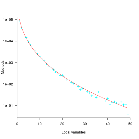
Approximately 50% of Java methods define five or fewer local variables. The plot below shows the number of Java methods defining a given number of local variables; the fitted regression equation, red line, has the form  , where
  is the number of local variables (code+data):
The reason most method define few local variables is that most methods only contain a few lines. The plot below shows the number of Java methods containing an estimated number of lines of code; the fitted regression equation, red line, has the form  , where
  is estimated lines of code (code+data):
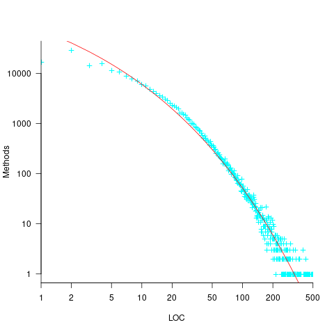
The plot below shows the number of local variables against estimated lines of code in the corresponding method; the fitted regression equation, red line, has the form  , where
  is the number of local variables (code+data):
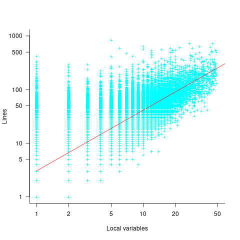
The strong connection between the number of lines of code and number of local variables in a method means that these two factors are effectively interchangeable in a regression model.
A local variable name is likely to be chosen before all, or even any, of the code that uses it is written. The hypothesis that the choice of a variable name is influenced by the length of a method, or the span of lines over which the variable is used, assumes some degree of foresight on the part of the developer.
The cited papers posed the question at the start of this post, and I built a variety of regression models looking to find those factors that are the best predictors of the length of the name (measured in characters or number of subcomponents), or the extent to which the length of the name predicted the amount of code over which it was used (either as a percentage or actual number of lines). Factors used include: order of variable definition in function, percentage of method code over which variable was used. See code+data.
The better models explained up to around 5% of the variance in the data. So there is an effect, but it’s very small. For instance, the model , where
  is the number of lines between variable definition and its last use, and
  is the number of characters in its name, is effectively a relationship between the mean value of these two factors that captures some of the variance around their means.
Motivation and software development
If people were not motivated to write software, computers would not have anything to do. What motivates a person to write software?
The source of human motivation may be intrinsic, as when pleasure is derived from performing the activity, or it may be extrinsic, such as being paid.
For some developers, writing software is a hedonistic activity. Intrinsic motivation continues to be the attractive force behind very many Open source projects.
People have to make a living, and being paid to write software creates an extrinsic motivation.
What do we know about human motivation?
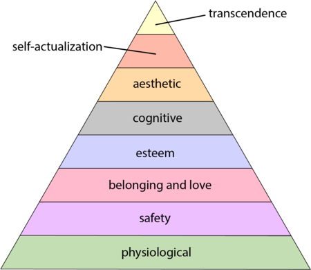
The 1943 paper A Theory of Human Motivation introduced Maslow’s hierarchy of needs, which is now often used as a structure for thinking about motivation. The image below, from Wikipedia, shows Maslow’s hierarchy:
Managers have long known that various kinds of carrots & sticks can be used to incentivize people to behave in a particular way, i.e., applying extrinsic motivation.
Incentives are actively researched in business and marketing departments. Unfortunately, sometimes more fashionable topics, such as cognitive biases, divert researcher’s interest.
Despite its fundamental importance, developer motivation is rarely considered, let alone a subject of research, within computing departments.
As purveyors of intangible goods, the software industry is aware of many issues around motivation. Managers of software teams appreciate the impact of team motivation on performance. Team motivation is a perennial topic of discussion for the Agile coaches and Scrum masters I meet. Companies selling products offering an API hire developer evangelists, whose job is to motivate third-party developers to use this API.
Software systems that continue to be used become part of the fabric of larger, more complex, systems. The motivations of the inhabitants of complex systems can have many unintended consequences.
Motivation is an intangible that cannot be measured directly; its effect has to be inferred from the results produced by the behaviors it drives. Distinguishing between two diametrically different motivations can present a conundrum, e.g., distinguishing between developers following Parkinson’s law or striving to meet a deadline.
Books don’t usually have much to say about the human side of software product management. A well-known exception is Peopleware: Productive Projects and Teams.
My evidence-based software engineering book should have had a chapter devoted to motivation, but given its focus on publicly available data, I had to make do with several 1-page subsections.
Accuracy of Function Point estimates
The number of Function points, FP, contained in the implementation of a software system are counted by following a specified counting process. The number of FP counted for a project is mapped to a cost estimate by multiplying the number of FP by the predetermined cost value of one FP; the predetermined value is based on cost data from similar previous projects within the company. The FP process is so popular as a unit of cost estimation that there are six different ISO standards specifying six different Function point measurement processes.
TL;DR: Estimated cost is not as accurate as traditional time based estimating, although the estimation process may produce consistent FP counts.
The FP certification schemes run by various organizations require applicants to pass exams that check they are consistently following the specified processes to produce consistent FP counts, i.e., that certified practitioners give very similar answers for the same implementation problem. Experiments where subjects used different counting processes to count FP for the same task, have found what looks like a linear relationship between various pairs of FP counting processes.
Having certified FP employees/consultants produce similar counts is all well and good, but what management actually wants is a close correspondence between estimated and actual costs. What does the available data show with regard to FP cost estimation accuracy?
I know of two FP/Cost datasets, one containing 149 points from one company (actual costs have been normalised), and the other 492 points from three companies (actual costs in Euros; FP used is IFPUG); this dataset also includes additional context information and is used in this post’s analysis.
What is the relationship between an estimate based on FP and actual cost? The plot below show FP against actual cost, the red line is the fitted regression equation  , the grey line shows
  (code+data):
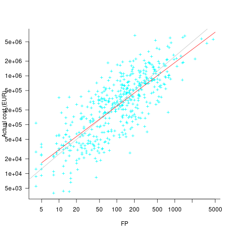
The power law exponent, 0.8, is slightly smaller than the 0.85 value found when fitting time estimates to actual times.
The dataset includes information specifying: anonymous organization ID, development method (78.5% plan driven and 21.5% Scrum), business domain (e.g., Call center, Mortgages, Front office), and various 0/1 flags each denoting a particular characteristic.
Including this information in a regression model finds that some of them have an impact on the FP to actual cost mapping. This is not surprising, since the FP/cost mapping is intended to be based on similar previous projects. The fitted model has the form:

where:  ,
,  ,
,  , and
, and  are constants for the corresponding items from the fitted regression model.
The fitted value for the scrum the development method is  , and
, and  for plan based (i.e., waterfall), i.e., Agile FP are cheaper than Waterfall FP. The idea of using both FP and scrum had not crossed my mind. Estimating via FP requires a detailed breakdown of the work to be done, while scrum is a process that discovers the work to be done. Perhaps a scrum like methodology was used to implement the detailed breakdown used to count FPs. The apparent lower cost of scrum FPs could just be a result of discovering that some planned functionality was not required.
How accurate were the FP estimates?
It is not possible to answer this question between we don’t know the cost assigned to one FP; in the above plot, the grey lines shows  .
.
We can calculate an estimate accuracy relative to the fitted model (the red line above). The mapping from FP to cost can vary between organizations, and the following analysis is based on the data for each distinct organization. The plot below shows the points, and associated fitted regression line, for the three organizations (code+data):
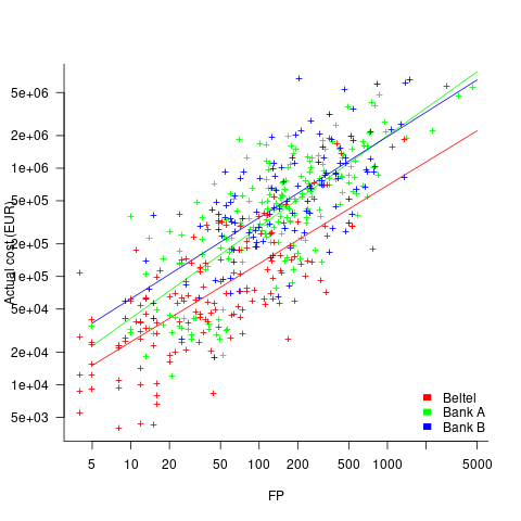
Each organization’s fitted regression model can be used to calculate confidence intervals. Approximately 68% of FP estimates could be off by over a factor two (between 2.3 and 2.5) from the mean actual cost, while for the 95% interval FP estimates could be off by over a factor five (it varied between 5.0 and 5.8); code+data. The corresponding factors for traditional developer time estimation are two and four.
The exponent varies between 0.72 and 0.84, with Beltel and Bank B having very similar values (the exponent for time estimates is often close to 0.85). The FP/Cost mapping is likely to be similar for the two banks, but lower for the telecoms company.
Does slicing the data by organization and business domain reduce the width of the confidence intervals, i.e., smaller multiplication factor? In some cases the width is reduced, but in other cases the width is increased; the 68% factor is between 1.9 and 3.1, the 95% factor is between 3.2 and 9.4.
Who are the famous academics in software engineering?
Who are today’s ‘famous’ academics in software engineering?
Famous as in, you can mention their name when chatting with general software developers, and expect those present to have heard of them, or you have heard their names dropped into a conversation, say, at least 3+ times this year (I’m excluding academics who are famous within one specific niche of software engineering). Academic, as in, works in an institution of secondary or tertiary higher learning.
When I started out in industry, the works of Knuth and Dijkstra were cited (not always accurately), people would talk about Ted Codd’s latest position on how best to structure a database. Tony Hoare later became known through his books, and Leslie Lamport for distributed systems and perhaps LaTeX. In very large niches, William Kahan for numerical analysis, and Barbara Liskov for the Liskov substitution principle.
Anyone suggesting Kernighan and Ritchie, of C and Unix fame, is overlooking the fact they worked in an industrial research lab.
A book series continues to maintain Knuth’s fame, while Dijkstra kept himself in the news by being a source of controversial quotes for industry journalists, and for kicking off the Go-To statement considered harmful debate (the latter is likely the reason that anybody has heard of him today). Has Kahan escaped his niche, even though use of floating-point arithmetic is now perhaps even more niche than it used to be?
How might academics become famous?
Widely used algorithms/metrics/techniques named after a person generates a kind of anonymous name recognition. For instance, Halstead complexity metric and McCabe’s cyclomatic complexity metric, and from the 1990s Shor’s algorithm.
Some people achieve fame through their association with a language. Academic name/language pairs include: McCarthy/Lisp, Wirth/Pascal, Stroustrup/C++ (worked in industry, university, industry, university), Peyton Jones/Haskell (university, industrial research, industry), Leroy/OCaml, Meyer/Eiffel.
An influential book, or widely read blog can generate a kind of fame.
Many academics have written an ‘algorithms’ book, and readers may have fond memories of the particular book they used as an undergraduate. Barry Boehm wrote “Software Engineering Economics”, but is more likely to be known for the model he spent his life promoting, i.e., the COCOMO model.
Fred Brooks, author of one of the most famous books in software engineering The Mythical Man Month, was not an academic worked in industry and then academia.
I have always been surprised by how many Turing award winners I have never heard of, or while recognizing a name am completely unfamiliar with their work. I am less surprised by my failure to recognise around half the names in the Wikipedia category software engineering researchers.
A few people are known because of the widespread use of their software (Linus Torvalds has never been an academic). Richard Stallman, employed as an academic, originally became famous as the author of the GNU version of emacs and gcc; the fame from the Free Software Foundation came after copyleft took off.
Are there academics who have become ‘famous’ in software engineering this century? I’m not in a position to answer this because I don’t read introductory software books, and generally avoid bike-shed discussions.
Does the resurgence of interest in AI mean that Judea Pearl’s fame is no longer niche?
I do read recent academic papers, and the only person on the list of most frequently cited authors in my evidence-based software engineering book with any claim to fame, researches cognitive neuroscience, i.e., Stanislas Dehaene.
Is software engineering a field where it is possible for a person, academic or otherwise, to become famous?
If there are fame worthy discoveries waiting to be made, or fame worthy software engineering book waiting to be written, how likely is it that the people responsible will be academics? A lot of the advances in software engineering have been made and continue to be made by those working in industry.
Suggestions relating to (in)famous academics welcome.
Benchmarking fuzzers
Fuzzing has become a popular area of research in the reliability & testing community, with a stream of papers claiming to have created a better tool/algorithm. The claims of ‘betterness’, made by the authors, often derive from the number of previously unreported faults discovered in some collection of widely used programs.
Developers in industry will be interested in using fuzzing if it provides a cost-effective means of discovering coding mistakes that are likely to result in customers experiencing a serious fault. This requirement roughly translates to: minimal cost for finding maximal distinct mistakes (finding the same mistake more than once is wasted effort); whether a particular coding mistake is likely to produce a serious customer fault is a decision decided by people.
How do different fuzzing tools compare, when benchmarking the number of distinct mistakes they each find, for a given amount of cpu time?
TL;DR: I don’t know, and this approach is probably not a useful way of comparing fuzzers.
Fuzzing researchers are currently competing on the number of previously unreported faults discovered, i.e., not listed in the fuzzed program’s database of fault reports. Most research papers only report the number of distinct faults discovered in each program fuzzed, the amount of wall clock hours/days used (sometimes weeks), and the characteristics of the computer/cluster on which the campaign was run. This may be enough information to estimate an upper bound on faults per unit of cpu time; more detailed data is rarely available (I have emailed the authors of around a dozen papers asking for more detailed data).
A benchmark based on comparing faults discovered per unit of cpu time only makes sense when the new fault discovery rate is roughly constant. Experience shows that discovery time can vary by orders of magnitude.
Code coverage is a fuzzer performance metric that is starting to be widely used by researchers. Measures of coverage include: statements/basic blocks, conditions, or some object code metric. Coverage has the advantage of providing defined fuzzer objectives (e.g., generate input that causes uncovered code to be executed), and is independent of the number of coding mistakes present in the code.
How is a fuzzer likely to be used in industry?
The fuzzing process may be incremental, discovering a few coding mistakes, fixing them, rinse and repeat; or, perhaps fuzzing is run in a batch over, say, a weekend when the test machine is available.
The current research approach is batch based, not fixing any of the faults discovered (earlier researchers fixed faults).
Not fixing discovered faults means that underlying coding mistakes may be repeatedly encountered, which wastes cpu time because many fuzzers terminate the run when the program they are testing crashes (a program crash is a commonly encountered fuzzing fault experience). The plot below shows the number of occurrences of the same underlying coding mistake, when running eight fuzzers on the program JasPer; 77 distinct coding mistakes were discovered, with three fuzzers run over 3,000 times, four run over 1,500 times, and one run 62 times (see Green Fuzzing: A Saturation-based Stopping Criterion using Vulnerability Prediction by Lipp, Elsner, Kacianka, Pretschner, Böhme, and Banescu; code+data):
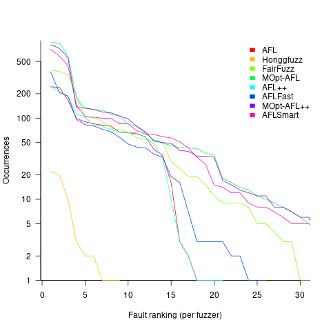
I have not seen any paper where the researchers attempt to reduce the number of times the same root cause coding mistake is discovered. Researchers are focused on discovering unreported faults; and with around 98% of fault discoveries being duplicates, appear to have resources to squander.
If developers primarily use a find/fix iterative process, then duplicate discoveries will be an annoying drag on cpu time. However, duplicate discoveries are going to make it difficult to effectively benchmark fuzzers.
Research ideas for 2023/2024
Students sometimes ask me for suggestions of interesting research problems in software engineering. A summary of my two recurring suggestions, for this year, appears below; 2016/2017 and 2019/2020 versions.
How many active users does a program or application have?
The greater the number of users, the greater the number of reported faults. Estimates of program reliability have to include volume of usage as an integral part of the calculation.
Non-trivial amounts of public data on program usage is non-existent (in a few commercial environments, users are charged for using software on a per-usage basis, but this data is confidential). Usage has to be estimated by indirect means.
A popular indirect technique for estimating the popularity of Github repos is to count the number of stars it has; however, stars have a variety of interpretations. The extent to which Github stars tracks usage of the repo’s software is not known.
Other indirect techniques include: web server logs, installs of the application, or the operating system.
One technique that has not yet been researched is to make use of the identity of those reporting faults. A parallel can be drawn with the fish population in lakes, which is not directly visible. Ecologists have developed techniques for indirectly estimating the population size of distinct creatures using information about a subset of the population, and some of the population models developed for ecology can be adapted to estimating program user populations.
Estimates of population size can be obtained by plugging information on the number of different people reporting faults, and the number of reports from the same person into these models. This approach is not as easy as it sounds because sometimes the same person has multiple identities, reported faults also need to be deduplicated and cleaned (30-40% of reports have been found to be requests for enhancements).
Nested if-statement execution
As if-statement nesting depth increases, the number of conditions controlling the execution of the enclosed code increases.
Being able to estimate the likelihood of executing the code controlled by an if-statement is of interest to: compilers wanting to target optimizations along the most frequently executed paths, special handling for error paths, testing along the least/most likely paths (e.g., fuzzers wanting to know the conditions needed to reach a given block), those wanting to organize code for ease of understanding, by reducing cognitive effort to understand.
Possible techniques for analysing the likelihood of executing code controlled by one or more nested if-statements include:
- Compiler writers have discovered various heuristics for predicting the likely outcome of a branch, and there are probably more to be discovered. Statement coverage counts provides a ground truth against which to compare ideas,
- analysis of the conditional expression,
- mathematical analysis of the distribution of values of variables in conditional expressions.
The lifetime of performance coding issues
Coding activities that a developer might spend time on include: adding new functionality, fixing a reported fault, or fiddling with existing code with the intent of making it ‘better’ in some sense (which these days goes by the catch-all name of refactoring).
Improving performance, e.g., changing software to use less cpu/memory is considered, by developers, to make it ‘better’ (whether users are likely to notice the difference, or management see a ROI is for another article). There is a breed of developer whose DNA encodes for pleasure receptors that are only fire when working to reduce the amount of cpu/memory used by a program.
The paper Characterizing the evolution of statically-detectable performance issues of Android Apps by Das, Di Penta, and Malavolta studied the creation/removal of nine distinct performance coding issues in the source of 316 Android Apps (118 Apps contained five or more issues); a total of 2,408 performance issues were tracked.
What patterns might be present in the paper’s performance issues data?
I would expect there to be more creations in Apps containing more code, and more removals the longer an App is maintained; both very obvious. With more developers working on an App, there are going to be more creations and removals; do they cancel out? Management might decide to invest time in performance improvements for the next release, which would cause a spike in the number of removals per unit time.
How long do the nine performance issues survive in code, before being removed? The plot below shows the Kaplan Meier survival curve for Apps containing at least five issues (dotted blue/green are the 95% confidence intervals, code+data):
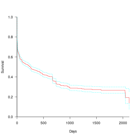
Around 15% of issues were removed on the day they are created, and by the eighth day around 30% had been removed. The roughly steady decline lasts for two-years, followed by almost stasis. Is two-years the active development lifetime of a successful Android App?
In isolation, the slope of the survival curve between eight days and two-years is not that interesting (it could be used to rule out models of the issue discovery process, e.g., happenstance discovery while working on other tasks). However, comparing it against the corresponding survival curve for reported faults tells us something about developer/management investment priorities for the two kinds of tasks, as measured by time to fix (which is a proxy for effort invested).
Unfortunately, this study did not collect information on coding mistake lifetimes, or time between a fault being reported and fixed. There have been studies investigating the survival time of coding mistakes. Reported faults should have the lowest survival rate, while the survival of coding mistakes will depend on the number of users (i.e., more users creates more opportunities to experience a fault and report it).
What factors influence performance issue time-to-fix?
The data includes information on the kind of performance issue, the number of times the App has been downloaded from the Google Play Store, and the number of contributors to the App.
Using these variables, a Cox proportional hazards model was fitted to model the survival time. In a proportional hazards model, the model coefficients are not absolute values, but provide ratio information. For instance, the following table shows the coefficients of the fitted model (code+data). Using these coefficients, we can compare the time taken to fix, say, a FloatMath issue relative to a ViewTag issue. The coefficient ratio  is the estimated ratio of fix times of the two respective issues.
Coefficient Standard error Performance issue FloatMath 0.64445 0.14175 HandlerLeak 0.69958 0.12736 Recycle 0.83041 0.11386 UseSparseArrays 0.73471 0.12493 UseValueOf 0.64263 0.11827 ViewHolder 0.87253 0.14951 ViewTag 5.24257 0.46500 Wakelock 3.34665 0.72014 Downloads 50-100 0.62490 0.26245 100-500 0.64699 0.22494 500-1000 0.56768 0.23505 1000-5000 0.50707 0.22225 5000-10000 0.53432 0.22486 10000-50000 0.62449 0.21626 50000-100000 0.42214 0.23402 100000-500000 0.21479 0.25358 1000000-5000000 0.40593 0.21851 10000000-50000000 0.03474 0.61827 100000000-500000000 0.30693 0.39868 1000000000-5000000000 0.41522 0.61599 NA 0.03868 1.02076 Contributors 1.04996 0.01265 |
There is not a lot of difference in the coefficients for the number of downloads (the model fit is poor when the Standard error is close to the Coefficient value).
The paper Investigating Types and Survivability of Performance Bugs in Mobile Apps analyses a smaller dataset of performance issue lifetimes.
Recent Comments