Archive
Lifetime of coding mistakes in the Linux kernel
What is the lifetime of coding mistakes in the Linux kernel? Some coding mistakes result in fault reports (some of which are fixed), while many are removed when the source that contains them is deleted/changed during ongoing development.
After fixing the coding mistake(s) in the kernel that generated a reported fault, developer(s) log the commit that introduced the coding mistake, along with the commit that fixed it. This logging started in 2013, and I only found out about it this week. To be exact, I discovered the repo: A dataset of Linux Kernel commits created by Maes Bermejo, Gonzalez-Barahona, Gallego, and Robles.
The log contains the commit hashes for the 90,760 fixes made to the 63 mainline kernel versions from 3.12 to 6.13. The complete log of 1,233,421 commits has to be searched to extract the details, e.g., date, lines added, etc.
The kernel development process involves regular release cycles of around 80 days. Developers submit the code they want to be included in the next release, this goes through a series of reviews, with Linus making the final decision.
The following analysis is based on the coding mistakes introduced between successive kernel releases, e.g., version 3.13 coding mistakes are those introduced into the source between 4 Nov 2013 (the day after version 3.12 was released) and 19 Jan 2014 (when version 3.13 was released). Code will have been worked on, and mistakes created/fixed, before it reached the kernel, which ensures some level of maturity.
The number of people working with pre-release code is likely to be tiny, compared to the number running released kernels. Consequently, the characteristics of coding mistake lifetime is expected to be different pre/post release, if only because more users are likely to report more faults.
The plot below shows the pre-release daily mistake fixed density against days since start of work on the current release, the red line is a fitted regression line mapped to density (fitted regression is a biexponential; code and data):
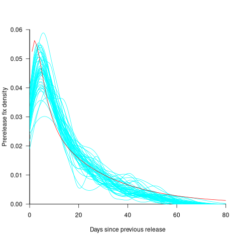
For all versions, the prior to release daily fix rate follows a consistent pattern: Most fixes occur in the first few days, with roughly an exponential decline to the release date.
The following analysis builds a broad brush model of cumulative fixes over time across 53 mainline kernel releases (the final 10 releases were not included because of their relatively short history).
The number of users of a new kernel takes time to increase as it percolates onto systems, e.g., adopted by Linux distributions and then installed by users, or installed by cloud providers. Eventually, code first included in a particular version will be running on most systems.
The post release daily fix rate is best modelled using the cumulative number of fixes, i.e., total number of fixes up to a given day since release. The models fitted below are based on dividing the post release cumulative fixes into before/after 200 days since release. The 200-day division is a round number (technically, a nearby value may provide a better fit) that supports the fitting of good quality before/after regression models. Averaged over all releases, 42% of fixes occurred within 200-days, and 58% after 200-days.
The plot below shows the cumulative number of post-release fixed faults, in red, for various kernel versions, with fitted regression lines in green and blue (grey line is at 200-days; code and data):

The equation fitted to the before 200-days fixes had the following form:
}")
where:  is a kernel version specific constant; see plot below.
The equation fitted to the after 200-days fixes had the following form:

where:  is a kernel version specific constant; see plot below.
Approximately, after release, the cumulative fix rate starts out quadratic in elapsed days, with the rate decreasing over time, until after 200-days the rate settles down to following the cube-root of days.
Comparing the number of post-release fixes across versions, there is a lot more variability in the first 200-days (i.e., the model fit to the data is sometimes very poor), relatively to after 200-days (where the model fit is consistently good).
Each kernel release has its own characteristics, parameterised by the values , and in the above equations. The plot below shows these values across versions, with red for , blue/green for , and grey line showing normalised LOC added/changed in the release (code and data):
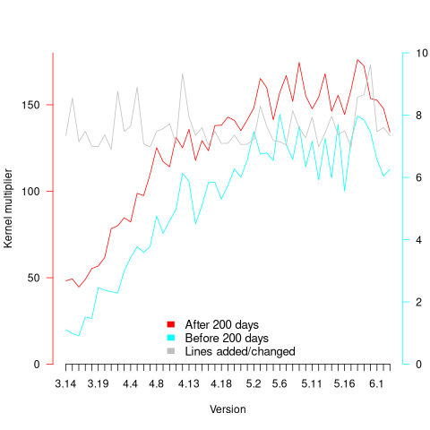
The plot clearly shows a large increase in the number of fixes between kernel version 3.14 and later versions. The before 200-days rate (blue/green) increase by a factor of seven, while the after 200-days rate increased by a factor of three.
Is this increase driven by some underlying factor in kernel development, or is it an external factor such as an increase in the number of users (more users leads to more faults reports), or the extensive post-release fuzz testing that is now common.
The number of lines of code added/changed, indicated by the grey line (shifted to fit plot axes) cannot be added to the fitted models because they exactly correlate with their respective version.
What is driving the long-term rate of fixes, i.e., cube-root of elapsed days?
Actually, what people are really want to know is what can be done to reduce the number of fixes required after release. When people ask me this, my usual reply is: “Spend more on testing”.
The probability of a coding mistake causing a fault report is decreasing: fixes reduce the number of remaining mistakes, and source added in one kernel version may be removed in a later version.
Perhaps the set of input behaviors is growing, producing the distinct conditions needed to trigger different coding mistakes, or the faults are occurring but are only reported when experienced by a small subset of users.
As always, more data is needed.
Decline in downloads of once popular packages
What happens to the popularity of Open source packages, measured in monthly downloads, once they cease to be updated or attract new users?
If the software does not have any competition within its domain, there is no reason why its popularity should decline. In practice, there are usually alternative packages offering the same or similar functionality. Even when alternatives are available, existing practice and sunk costs can slow migration. A year or so after I started using Asciidoc to write by Software Engineering book, the author announced that he was no longer going to update the software; initially there was no alternative, but the software did what I wanted, and I have been happily using it over the last 12 years.
The paper: Do All Software Projects Die When Not Maintained? Analyzing Developer Maintenance to Predict OSS Usage by Emily Nguyen measured the monthly downloads, commits and other characteristics of 38K GitHub packages having at least 10K downloads during any month between January 2015 and December 2020. The data made available (more here) is a subset, i.e., downloads for 1,583 projects starting in May 2015.
The author investigated the connection between various project characteristics (focusing on commits or lack thereof in particular) and downloads by fitting a Cox proportional hazards model.
The plot below shows the 67 monthly downloads for a selection of packages; the red line is a fitted local regression used to smooth the data (code and data):

Reasons for a decline from a peak number of downloads include: competition from alternative packages, change of fashion, and market saturation, or perhaps the peak was caused by a one-off event. Whatever the reason for a peak+decline, my interest is learning about patterns in the rate of decline.
Some of the monthly package downloads in the above plot have an obvious peak and decline, with others continually increasing, and others having multiple peaks. The following algorithm was used to select packages having a peak followed by a decline, based on the predicted values from a fitted loess model:
- find the month with the most downloads, this is the primary peak,
- if this month is within 10 months of the end of the measurement period, this is not a peak/decline package,
- does a secondary peak exist? A secondary peak is a month containing the most downloads from 10 months after the end of the primary peak, where the number of downloads is within 66% of the primary peak downloads,
- the secondary peak becomes the primary peak, provided it is not within 10 months of the end of the measurement period.
The final fraction of the primary peak is the average monthly download during the last three months divided by the peak month downloads.
The plot below shows the 693 packages whose final fraction of peak was below 0.6 against months from peak to the last month (at the end of 2020), with the red line showing a fitted regression of the form  (code and data):

As the above plot shows, there don’t appear to be any patterns in the decline of package downloads, and  is a poor predictor of fraction of peak.
Perhaps a more sophisticated peak+decline selection algorithm will uncover some patterns. Both ChatGPT (its generated python script failed) and Grok (very wrong answers) failed miserably at classifying the plots. Deepseek will only process images to extract text.
Occurrence of binary operator overloading in C++
Operator overloading, like many programming language constructs, was first supported in the 1960s (Algol 68 also provided a means to specify a precedence for the operator). C++ is perhaps the most widely used language supporting operator overloading; but not redefining their precedence.
I have always thought that operator overloading was more talked about than actually used (despite its long history, I have not been able to find any published usage information). A previous post noted that the CodeQL databases hosted by GitHub provides the data needed to measure usage, and having wrestled with the documentation (ql scripts used), C++ operator overload usage data is available.
The table below shows the total uses of overloaded and ‘usual’ binary operators in the source code (excluding headers) of 77 C++ repositories on GitHub (the 100 repositories C/C+ MRVA). The table is ordered by total occurrences of overloads, with the Percentage column showing the percentage use of overloaded operators against the total for the respective operator (i.e.,  ; code and data):
Binary Overload Usual Total Percentage << 103,855 20,463 124,318 83.5 == 21,845 118,037 139,882 15.6 != 14,749 69,273 84,022 17.6 * 12,849 57,906 70,755 18.2 + 10,928 103,072 114,000 9.6 && 8,183 64,148 72,331 11.3 - 5,064 77,775 82,839 6.1 <= 3,960 18,344 22,304 17.8 & 3,320 27,388 30,708 10.8 < 1,351 93,393 94,744 1.4 >> 1,082 11,038 12,120 8.9 / 1,062 29,023 30,085 3.5 > 537 44,556 45,093 1.2 >= 473 27,738 28,211 1.7 | 293 13,959 14,252 2.0 ^ 71 1,248 1,319 5.4 <=> 13 12 25 52.0 % 11 9,338 9,349 0.1 || 9 53,829 53,838 0.017 |
Use of the overloaded << operator is driven by standard library I/O, rather than left shifting.
There are seven operators where 10-20% of the usage is overloaded, which is a lot higher than I was expecting (not that I am a C++ expert).
How much does overloaded binary operator usage vary across projects? In the plot below, each vertical colored violin plot shows the distribution of overload usage for one operator across all 77 projects (the central black lines denote the range of the central 50% of the points; code and data):

While there is some variation between these 77 projects, in most cases a non-trivial percentage of an operator's usage is overloaded.
Fifth anniversary of Evidence-based Software Engineering book
Yesterday was the 5th anniversary of the publication of my book Evidence-based Software Engineering.
The general research trajectory I was expecting in the 2020s (e.g., more sophisticated statistical analysis and more evidence based studies) has been derailed by the arrival of LLMs three years ago. Almost all software engineering researchers have jumped on the LLM bandwagon, studying whatever LLM use case is likely to result in a published paper. While I have noticed more papers using statistical techniques discovered after the digital computer was invented (perhaps influenced by the second half of the book), there seems to be a lot fewer evidence based papers being published. I don’t expect researches studying software engineering to jump off the LLM bandwagon in the next few years.
The net result of this lack of new research findings is that the book contents are not yet in need of an update.
On a positive note, LLMs’ mathematical problem-solving capabilities have significantly reduced the time needed to analyse models of software engineering processes.
Had today’s LLMs been available while I was writing the book, the text would probably have included many more theoretical models and their analysis. ‘Probably’, because sometimes the analysis finds that a model does not provide meaningfully mimic reality, so it’s possible that only a few more models would have been included.
My plan for the next year is to use LLM’s mathematical problem-solving capabilities to help me analyse models of software engineering processes. A discussion of any interested results found will appear on this blog. I’m hoping that there will be active conversations on the evidence based software engineering Discord channel.
It makes sense to hone my model analysis skills by starting with the subject I am most familiar with, i.e., source code. It also helps that tools are available for obtaining more source measurement data.
I will continue to write about any interesting papers that appear on the arXiv lists cs.se and cs.PL, as well as the major conferences. There won’t be time to track the minor conferences.
Questions raised during model analysis sometimes suggest ideas that, when searched for, lead to new data being discovered. Discovering new data using a previously untried search phrase is always surprising.
Best tool for measuring lots of source code
Human written source code contains various common usage patterns. This blog has analysed a variety of these patterns, and in a few cases built models of processes that replicate these patterns. The data for this analysis has primarily comes from programs written in C and Java, because these are the languages that researchers most often study (tool availability and herd mentality).
Do these common usage patterns occur in other languages, or at least other C/Java like languages? I think so, and have set out to collect the necessary data. Obtaining this data requires large quantities of code written in many languages, and the ability to analyse code written in these languages.
GitHub contains huge quantities of code. There are two freely available source code analysis tools supporting many languages: Opengrep (the Open source version of semgrep) and CodeQL.
CodeQL’s method of operation had previously put me off trying it. The method is a two stage process: First a database of information is created by extracting information during a project’s build process (e.g., running existing makefiles and host compilers), followed by querying this database using a declarative language (think minimalist SQL with lots of built-in functions). This approach has the huge advantage of not having to worry about handling compiler dialects/options, however, I’m an ingrained user of tools that process individual files.
From the research perspective, CodeQL has a major feature that is not available with other tools. GitHub, who now owns CodeQL, host thousands of project databases and GitHub Actions allows third-parties to scan up to 1,000 databases of the most popular projects. Access to existing CodeQL databases removes the need to download repo/build project/store database locally.
CodeQL, like other static analysis tools, was designed to find issues/problems in code, and so might not support the kind of functionality I needed to extract source code measurements. The best way to find out if the data of interest could be extracted is to try and do it.
In the best developer tradition, I downloaded a prebuilt release (available for Linux, Windows and Mac; called CodeQL Bundles), skimmed the documentation, ran a simple QL script and spent an hour or two trying to figure out why I was getting Java runtime errors, e.g., “no String-argument constructor/factory method to deserialize from String value“.
Progress would have been faster if I had used Visual Studio Code, available free from the owners of GitHub, rather than the command line. The documentation is not command line oriented. Visual Studio handles details like creating a qlpack.yml file (whose necessary existence I eventually found out about). Also, the harmless looking metadata appearing in comments is necessary and had better match the output parameters of the query. How hard is it to warn that a file could not be found, or that metadata is missing?
The code databases are queried using the declarative language QL, which is a kind of minimal SQL (with the select appearing last, rather than first). The import statement specifies the language, or rather the name of a library module.
The imported library contains classes for each language construct (e.g., BlockStmt, Function, ArrayExpr, etc). In the query below, the line “from LocalScopeVariable lv” extracts all local scope variables, which can subsequently be referred to via the name lv. The where line lists conditions that must be met (in this example, not be a parameter and not be accessed; testing for unused variables). The select line invokes methods that return various kinds of information about the class, e.g., the name of the variable, and location within the source.
/** * @id compound-stmt * @kind problem * @problem.severity warning */ import cpp from LocalScopeVariable lv where not lv instanceof Parameter and not exists(lv.getAnAccess()) select "", ""+lv.getName()+ ","+lv.getLocation().getStartLine()+ ","+lv.getLocation().getEndLine()+ ","+lv.getEnclosingFunction()+","+bs.getFile() |
The output generated is driven by the select, whose number/kind of arguments must match that specified by the metadata.
Developers can write and call functions, such as this one:
predicate header_suffix(string fstr) { fstr = "h" or fstr = "H" or fstr = "hpp" } |
The QL language is a declarative logical query language with roots in Datalog (subset of Prolog). The claim that it is an object-oriented language is technically correct, in that it groups functions into things called classes and supports various constructs usually found in object-oriented languages. The language has the feel of an academic project that happened to be used in a tool that was in the right place at the right time. Using host compilers to enable the tool to support many languages must have been very attractive to GitHub.
Coding in a declarative logic language requires a major mindset change. There are no loops, if statements or assignments. The query is one, potentially very long and complicated, predicate. A mindset change is necessary, but not sufficient, some fluency with the library of functions available is also needed. For instance, the isSideEffectFree predicate is true/false, but does not return a value (so there is nothing to print). I wanted to output 0/1, depending on whether a function was side effect free or not. When asked, all the LLMs questioned insisted that QL supported if-statements and assignment, just like other languages. After lots of dead-ends, an LLM claimed that “CodeQL automatically treats boolean expressions in count as 1/0″, and a test run showed this to be the case:
count(int dummy | dummy = 1 and func.isSideEffectFree() | dummy) |
The QL scripts needed to extract all the data of immediate interest to me were easily implemented. Looking at existing scripts has given me some ideas for more patterns I might measure. CodeQL currently supports 10 languages, and their classes appear to be slightly different (my initial focus is C, C++, Java and Python).
Visual Studio Code is required to run multi-repository variant analysis, i.e., scan up to 1,000 project databases on GitHub. It was after installing the CodeQL extension that I discovered how much smoother the process is within this IDE, compared to the command line (and off course the output is slightly different). There may be alternatives to Visual Studio, but I’m sticking with what the official documentation says.
Stepping back, is CodeQL a useful tool?
For me it is currently very useful, because of the large number of project databases. Some practice is needed to achieve some fluency in the use of a declarative logic language, not a major hurdle.
The need to run queries against a project database may be a major inconvenience for some developers, depending on working practices. Those practicing continuous integration should be ok.
Recent Comments