Archive
Cognitive effort, whatever it might be
Software developers spend a lot of time acquiring knowledge and understanding of the software system they are working on. This mental activity fits within the field of Cognition, which covers all aspects of intellectual functions and processes. Human cognition as it related to software development is covered in chapter 2 of my book Evidence-based software engineering; a reading list.
Cognitive effort (e.g., thinking) is hard work, or at least mental effort feels like hard work. It has become fashionable for those extolling the virtues of some development technique/process to claim that one of its benefits is a reduction in cognitive effort; sometimes the term cognitive load is used, but I suspect this is not a reference to cognitive load theory (which is working memory based).
A study by Arai, with herself as the subject, measured the time taken to mentally multiply two four-digit values (e.g., 2,645 times 5,784). Over 2-weeks, Arai practiced on four days, on each day multiplying over 20 four-digit value pairs. A week later Arai multiplied 40 four-digit value pairs (starting at 1:45pm, finishing at 6:31pm), had dinner between 6:31-7:41 pm, and then, multiplied 20 four-digit value pairs (starting at 7:41, finishing at 10:07). The plot below shows the time taken for each mental multiplication sequence, with fitted regression lines (code+data):
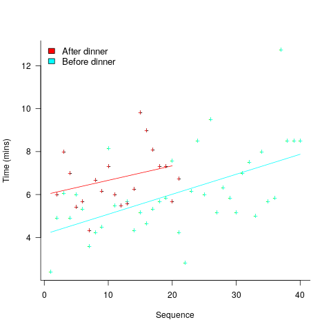
Over the course of the first, 5-hour session, average time taken slowed from four to eight minutes. The slope of the regression fit for the second session is poor, although the fit for the start value (6 minutes) is good.
The average increase in time taken is assumed to be driven by a reduction in mental effort, caused by the mental fatigue experienced during an extended period of continuous mental work.
What do we know about cognitive effort?
TL;DR Many theories and little evidence.
Cognitive psychologists are still at the stage of figuring out what exactly cognitive effort is. For instance, what is going on when we try harder (or decide to give up), and what is being conserved when we conserve our mental resources? The major theories include:
- Cognitive control: Mental processes form a continuum, from those that can be performed automatically with little or no effort, to those requiring concentrated conscious effort. Here, cognitive control is viewed as the force through which cognitive effort is exerted. The idea is that mental effort regulates the engagement of cognitive control in the same way as physical effort regulates the engagement of muscles.
- Metabolic constraints: Mental processes consume energy (glucose is the brain’s primary energy source), and the feeling of mental effort is caused by reduced levels of glucose. The extent to which mental effort is constrained by glucose levels is an ongoing debate.
- Capacity constraints: Working memory has a limited capacity (i.e., the oft quoted 7±2 limit), and tasks that fill this capacity do feel effortful. Cognitive load theory is based around this idea. A capacity limited working memory, as a basis of cognitive effort, suffers from the problem that people become mentally tired in the sense that later tasks feel like they require more effort. A capacity constrained model does not predict this behavior. Neither does a constraints model predict that increasing rewards can result in people exerting more cognitive effort.
How might cognitive effort be measured?
TL;DR It’s all relative or not at all.
To date, experiments have compared relative expenditure of effort between different tasks (some comparing cognitive with physical effort, other purely cognitive). For instance, showing that subjects are willing to perform a task requiring more cognitive effort when the expected reward is higher.
As always with human experiments, people can have very different behavioral characteristics. In particular, people differ in what is known as need for cognition, i.e., their willingness to invest cognitive effort.
While a lot of research has investigated the characteristics of working memory, the only real metric studied has been capacity, e.g., the longest sequence of digits that can be remembered/recalled, or span tasks involving having to remember words while performing simple arithmetic operations.
Experimental research on cognitive effort seems to be picking up, but don’t hold your breadth for reliable answers. Research of human characteristics can start out looking straight forward, but tends to quickly disappear down multiple, inconclusive rabbit holes.
Rounding and heaping in non-software estimates
Round numbers are often preferred in software task estimation times, e.g., 1, 5, 7 (hours in one working day), and 14. This human preference for round numbers is not specific to software, or to estimating. Round numbers can act as goals, as clustering points, may be used more often as uncertainty increases, or be the result of satisficing, etc.
Rounding can occur in response to any question involving a numeric value, e.g., a government census or survey asking citizens about their financial situation or health. Rounding introduces error in the analysis of data. The Whipple index, described in 1919, was the first attempt to quantify the amount of error; calculated as: “per cent which the number reported as multiples of 5 forms of one-fifth of the total number between ages 23 to 62 years inclusive.” for errors of reported age. Other metrics for this error have been proposed, and packages to calculate them are available.
At some point (the evidence suggests a 1940 paper) a published paper introduced the term heaping effect. These days, heaping is more often used to name the process, compared to rounding, e.g., heaping of values; ‘heaping’ papers do use the term rounding, but I have not seen ’rounding’ papers use heaping.
The choice of rounding values depends on the unit of measurement. For instance, reported travel arrival/departure times are rounded to intervals of 5, 14, 30 and 60 minutes; based on reported/actual travel times it is possible to estimate the probability that particular rounding intervals have been used.
The Whipple index fails when all the values are large (e.g., multiple thousands), or take a small range of values (e.g., between one and twenty).
One technique for handling rounding of large values is to define roundedness in terms of the fraction of value digits that are trailing zeroes. The plot below shows the number of households having a given estimated balance on their first mortgage in the 2013 Survey of Consumer Finances (in red), and the distribution of actual balances reported by the New York Federal Reserve (in blue/green; data extracted from plot in a paper and scaled to equalize total mortgage values; code+data):
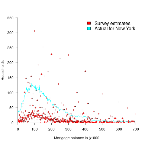
The relatively high number of distinct round numbers swamps any underlying distribution of actual values. While some values having some degree of roundness occur more often than non-round values, they still appear less often than expected by the known distribution. It is possible that homeowners have mortgages at round values because they of banking limits, or reasons other than rounding when answering the survey.
The plot below shows the number of people reporting having a given number of friends, plus number of cigarettes smoked per day, from the 2015 survey of Objective and Subjective Quality of Life in Poland (code+data):
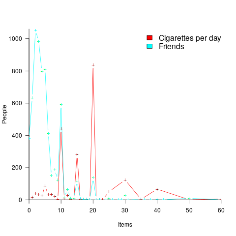
The narrow range of a person’s number of friends prevents the Whipple index from effectively detecting rounding/heaping.
The dominance of round numbers in the cigarettes smoked per day may be caused by the number of cigarettes contained in a packet, i.e., people may be accurately reporting that they smoke the contents of a packet, rather than estimating a rounded number.
Simple techniques are available for correcting the mean/variance when values are always rounded to specified boundaries. When the probability of rounding is not 100%, the calculation is more complicated.
Rounded/Heaped data contains multiple distributions, i.e., the non-rounded values and the rounded values; various mixture models have been proposed to fit such data. Alternatively, the data can be ‘deheaped’, and various deheaping techniques have been proposed.
Given the prevalence of significant amounts of rounding/heaping, it’s surprising how few people know about it.
Complex software makes economic sense
Economic incentives motivate complexity as the common case for software systems.
When building or maintaining existing software, often the quickest/cheapest approach is to focus on the features/functionality being added, ignoring the existing code as much as possible. Yes, the new code may have some impact on the behavior of the existing code, and as new features/functionality are added it becomes harder and harder to predict the impact of the new code on the behavior of the existing code; in particular, is the existing behavior unchanged.
Software is said to have an attribute known as complexity; what is complexity? Many definitions have been proposed, and it’s not unusual for people to use multiple definitions in a discussion. The widely used measures of software complexity all involve counting various attributes of the source code contained within individual functions/methods (e.g., McCabe cyclomatic complexity, and Halstead); they are all highly correlated with lines of code. For the purpose of this post, the technical details of a definition are glossed over.
Complexity is often given as the reason that software is difficult to understand; difficult in the sense that lots of effort is required to figure out what is going on. Other causes of complexity, such as the domain problem being solved, or the design of the system, usually go unmentioned.
The fact that complexity, as a cause of requiring more effort to understand, has economic benefits is rarely mentioned, e.g., the effort needed to actively use a codebase is a barrier to entry which allows those already familiar with the code to charge higher prices or increases the demand for training courses.
One technique for reducing the complexity of a system is to redesign/rework its implementation, from a system/major component perspective; known as refactoring in the software world.
What benefit is expected to be obtained by investing in refactoring? The expected benefit of investing in redesign/rework is that a reduction in the complexity of a system will reduce the subsequent costs incurred, when adding new features/functionality.
What conditions need to be met to make it worthwhile making an investment,  , to reduce the complexity,
  , of a software system?
Let’s assume that complexity increases the cost of adding a feature by some multiple (greater than one). The total cost of adding  features is:

where:  is the system complexity when feature
  is added, and
  is the cost of adding this feature if no complexity is present.
 ,
,  , …
, … 
where:  is the base complexity before adding any new features.
Let’s assume that an investment, , is made to reduce the complexity from  (with
(with  ) to
) to  , where
  is the reduction in the complexity achieved. The minimum condition for this investment to be worthwhile is that:
 or
or 
where:  is the total cost of adding new features to the source code after the investment, and
  is the total cost of adding the same new features to the source code as it existed immediately prior to the investment.
Resetting the feature count back to  , we have:
*F_1+(C_B+C_N+C_2)*F_2+...+(C_B+C_N+C_m)*F_m")
and
*F_1+(C_B+C_N-C_R+C_2)*F_2+...+(C_B+C_N-C_R+C_m)*F_m")
and the above condition becomes:
-(C_B+C_N-C_R+C_1))*F_1+...+((C_B+C_N+C_m)-(C_B+C_N-C_R+C_m))*F_m")


The decision on whether to invest in refactoring boils down to estimating the reduction in complexity likely to be achieved (as measured by effort), and the expected cost of future additions to the system.
Software systems eventually stop being used. If it looks like the software will continue to be used for years to come (software that is actively used will have users who want new features), it may be cost-effective to refactor the code to returning it to a less complex state; rinse and repeat for as long as it appears cost-effective.
Investing in software that is unlikely to be modified again is a waste of money (unless the code is intended to be admired in a book or course notes).
A new career in software development: advice for non-youngsters
Lately I have been encountering non-young people looking to switch careers, into software development. My suggestions have centered around the ageism culture and how they can take advantage of fashions in software ecosystems to improve their job prospects.
I start by telling them the good news: the demand for software developers outstrips supply, followed by the bad news that software development culture is ageist.
One consequence of the preponderance of the young is that people are heavily influenced by fads and fashions, which come and go over less than a decade.
The perception of technology progresses through the stages of fashionable, established and legacy (management-speak for unfashionable).
Non-youngsters can leverage the influence of fashion’s impact on job applicants by focusing on what is unfashionable, the more unfashionable the less likely that youngsters will apply, e.g., maintaining Cobol and Fortran code (both seriously unfashionable).
The benefits of applying to work with unfashionable technology include more than a smaller job applicant pool:
- new technology (fashion is about the new) often experiences a period of rapid change, and keeping up with change requires time and effort. Does somebody with a family, or outside interests, really want to spend time keeping up with constant change at work? I suspect not,
- systems depending on unfashionable technology have been around long enough to prove their worth, the sunk cost has been paid, and they will continue to be used until something a lot more cost-effective turns up, i.e., there is more job security compared to systems based on fashionable technology that has yet to prove their worth.
There is lots of unfashionable software technology out there. Software can be considered unfashionable simply because of the language in which it is written; some of the more well known of such languages include: Fortran, Cobol, Pascal, and Basic (in a multitude of forms), with less well known languages including, MUMPS, and almost any mainframe related language.
Unless you want to be competing for a job with hordes of keen/cheaper youngsters, don’t touch Rust, Go, or anything being touted as the latest language.
Databases also have a fashion status. The unfashionable include: dBase, Clarion, and a whole host of 4GL systems.
Be careful with any database that is NoSQL related, it may be fashionable or an established product being marketed using the latest buzzwords.
Testing and QA have always been very unsexy areas to work in. These areas provide the opportunity for the mature applicants to shine by highlighting their stability and reliability; what company would want to entrust some young kid with deciding whether the software is ready to be released to paying customers?
More suggestions for non-young people looking to get into software development welcome.
Evaluating estimation performance
What is the best way to evaluate the accuracy of an estimation technique, given that the actual values are known?
Estimates are often given as point values, and accuracy scoring functions (for a sequence of estimates) have the form }") , where is the number of estimated values,
, where is the number of estimated values,  the estimates, and
  the actual values; smaller
  is better.
Commonly used scoring functions include:
=(E-A)^2") , known as squared error (SE)
, known as squared error (SE)=delim{|}{E-A}{|}") , known as absolute error (AE)
, known as absolute error (AE)=delim{|}{E-A}{|}/A") , known as absolute percentage error (APE)
, known as absolute percentage error (APE)=delim{|}{E-A}{|}/E") , known as relative error (RE)
, known as relative error (RE)
APE and RE are special cases of: =delim{|}{1-(A/E)^{beta}}{|}") , with
, with  and
and  respectively.
Let’s compare three techniques for estimating the time needed to implement some tasks, using these four functions.
Assume that the mean time taken to implement previous project tasks is known,  . When asked to implement a new task, an optimist might estimate 20% lower than the mean,
  , while a pessimist might estimate 20% higher than the mean,
  . Data shows that the distribution of the number of tasks taking a given amount of time to implement is skewed, looking something like one of the lines in the plot below (code):
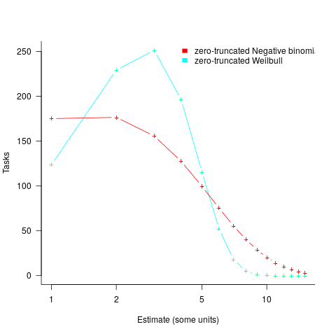
We can simulate task implementation time by randomly drawing values from a distribution having this shape, e.g., zero-truncated Negative binomial or zero-truncated Weibull. The values of  and
and  are calculated from the mean, , of the distribution used (see code for details). Below is each estimator’s score for each of the scoring functions (the best performing estimator for each scoring function in bold; 10,000 values were used to reduce small sample effects):
    SE   AE   APE   RE

  2.73 1.29 0.51 0.56

 2.31 1.23 0.39 0.68

  2.70 1.37 0.36 0.86
Surprisingly, the identity of the best performing estimator (i.e., optimist, mean, or pessimist) depends on the scoring function used. What is going on?
The analysis of scoring functions is very new. A 2010 paper by Gneiting showed that it does not make sense to select the scoring function after the estimates have been made (he uses the term forecasts). The scoring function needs to be known in advance, to allow an estimator to tune their responses to minimise the value that will be calculated to evaluate performance.
The mathematics involves Bregman functions (new to me), which provide a measure of distance between two points, where the points are interpreted as probability distributions.
Which, if any, of these scoring functions should be used to evaluate the accuracy of software estimates?
In software estimation, perhaps the two most commonly used scoring functions are APE and RE. If management selects one or the other as the scoring function to rate developer estimation performance, what estimation technique should employees use to deliver the best performance?
Assuming that information is available on the actual time taken to implement previous project tasks, then we can work out the distribution of actual times. Assuming this distribution does not change, we can calculate APE and RE for various estimation techniques; picking the technique that produces the lowest score.
Let’s assume that the distribution of actual times is zero-truncated Negative binomial in one project and zero-truncated Weibull in another (purely for convenience of analysis, reality is likely to be more complicated). Management has chosen either APE or RE as the scoring function, and it is now up to team members to decide the estimation technique they are going to use, with the aim of optimising their estimation performance evaluation.
A developer seeking to minimise the effort invested in estimating could specify the same value for every estimate. Knowing the scoring function (top row) and the distribution of actual implementation times (first column), the minimum effort developer would always give the estimate that is a multiple of the known mean actual times using the multiplier value listed:
                   APE   RE

Negative binomial  1.4   0.5

Weibull            1.2   0.6
For instance, management specifies APE, and previous task/actuals has a Weibull distribution, then always estimate the value  .
.
What mean multiplier should Esta Pert, an expert estimator aim for? Esta’s estimates can be modelled by the equation ") , i.e., the actual implementation time multiplied by a random value uniformly distributed between 0.5 and 2.0, i.e., Esta is an unbiased estimator. Esta’s table of multipliers is:
, i.e., the actual implementation time multiplied by a random value uniformly distributed between 0.5 and 2.0, i.e., Esta is an unbiased estimator. Esta’s table of multipliers is:
                   APE     RE

Negative binomial  1.0   0.7

Weibull                     1.0     0.7
A company wanting to win contracts by underbidding the competition could evaluate Esta’s performance using the RE scoring function (to motivate her to estimate low), or they could use APE and multiply her answers by some fraction.
In many cases, developers are biased estimators, i.e., individuals consistently either under or over estimate. How does an implicit bias (i.e., something a person does unconsciously) change the multiplier they should consciously aim for (having analysed their own performance to learn their personal percentage bias)?
The following table shows the impact of particular under and over estimate factors on multipliers:
                 0.8 underestimate bias   1.2 overestimate bias

Score function          APE   RE            APE   RE

Negative binomial        1.3   0.9           0.8   0.6

Weibull                 1.3       0.9           0.8   0.6
Let’s say that one-third of those on a team underestimate, one-third overestimate, and the rest show no bias. What scoring function should a company use to motivate the best overall team performance?
The following table shows that neither of the scoring functions motivate team members to aim for the actual value when the distribution is Negative binomial:
                    APE      RE

Negative binomial    1.1     0.7

Weibull                               1.0       0.7
One solution is to create a bespoke scoring function for this case. Both APE and RE are special cases of a more general scoring function (see top). Setting  in this general form creates a scoring function that produces a multiplication factor of 1 for the Negative binomial case.
Twitter and evidence-based software engineering
This year’s quest for software engineering data has led me to sign up to Twitter (all the software people I know, or know-of, have been contacted, and discovery through articles found on the Internet is a very slow process).
@evidenceSE is my Twitter handle. If you get into a discussion and want some evidence-based input, feel free to get me involved. Be warned that the most likely response, to many kinds of questions, is that there is no data.
My main reason for joining is to try and obtain software engineering data. Other reasons include trying to introduce an evidence-based approach to software engineering discussions and finding new (to me) problems that people want answers to (that are capable of being answered by analysing data).
The approach I’m taking is to find software engineering tweets discussing a topic for which some data is available, and to jump in with a response relating to this data. Appropriate tweets are found using the search pattern: (agile OR software OR "story points" OR "story point" OR "function points") (estimate OR estimates OR estimating OR estimation OR estimated OR #noestimates OR "evidence based" OR empirical OR evolution OR ecosystems OR cognitive). Suggestions for other keywords or patterns welcome.
My experience is that the only effective way to interact with developers is via meaningful discussion, i.e., cold-calling with a tweet is likely to be unproductive. Also, people with data often don’t think that anybody else would be interested in it, they have to convinced that it can provide valuable insight.
You never know who has data to share. At a minimum, I aim to have a brief tweet discussion with everybody on Twitter involved in software engineering. At a minute per tweet (when I get a lot more proficient than I am now, and have workable templates in place), I could spend two hours per day to reach 100 people, which is 35,000 per year; say 20K by the end of this year. Over the last three days I have managed around 10 per day, and obviously need to improve a lot.
How many developers are on Twitter? Waving arms wildly, say 50 million developers and 1 in 1,000 have a Twitter account, giving 50K developers (of which an unknown percentage are active). A lower bound estimate is the number of followers of popular software related Twitter accounts: CompSciFact has 238K, Unix tool tips has 87K; perhaps 1 in 200 developers have a Twitter account, or some developers have multiple accounts, or there are lots of bots out there.
I need some tools to improve the search process and help track progress and responses. Twitter has an API and a developer program. No need to worry about them blocking me or taking over my business; my usage is small fry and I’ not building a business to take over. I was at Twitter’s London developer meetup in the week (the first in-person event since Covid) and the youngsters present looked a lot younger than usual. I suspect this is because the slightly older youngsters remember how Twitter cut developers off at the knee a few years ago by shutting down some useful API services.
The Twitter version-2 API looks interesting, and the Twitter developer evangelists are keen to attract developers (having ‘wiped out’ many existing API users), and I’m happy to jump in. A Twitter API sandbox for trying things out, and there are lots of example projects on Github. Pointers to interesting tools welcome.
Evidence-based Software Engineering: now in paperback form
I made my Evidence-based Software Engineering book available as a pdf file. While making a printed version available looked possible, I was uncertain that the result would be of acceptable quality; the extensive use of color and an A4 page size restricted the number of available printers who could handle it. Email exchanges with several publishers suggested that the number of likely print edition copies sold would be small (based on experience with other books, under 100). The pdf was made available under a creative commons license.
Around half-million copies of the pdf have been downloaded (some partially).
A few weeks ago, I spotted a print version of this book on Amazon (USA). I have no idea who made this available. Is the quality any good? I was told that it was, so I bought a copy.
The printed version looks great, with vibrant colors, and is reasonably priced. It sits well in the hand, while reading. The links obviously don’t work for the paper version, but I’m well practised at using multiple fingers to record different book locations.
I have one report that the Kindle version doesn’t load on a Kindle or the web app.
If you love printed books, I heartily recommend the paperback version of Evidence-based Software Engineering; it even has a 5-star review on Amazon 😉
Programming language similarity based on their traits
A programming language is sometimes described as being similar to another, more wide known, language.
How might language similarity be measured?
Biologists ask a very similar question, and research goes back several hundred years; phenetics (also known as taximetrics) attempts to classify organisms based on overall similarity of observable traits.
One answer to this question is based on distance matrices.
The process starts by flagging the presence/absence of each observed trait. Taking language keywords (or reserved words) as an example, we have (for a subset of C, Fortran, and OCaml):
if then function for do dimension object C 1 1 0 1 1 0 0 Fortran 1 0 1 0 1 1 0 OCaml 1 1 1 1 1 0 1 |
The distance between these languages is calculated by treating this keyword presence/absence information as an n-dimensional space, with each language occupying a point in this space. The following shows the Euclidean distance between pairs of languages (using the full dataset; code+data):
C Fortran OCaml C 0 7.615773 8.717798 Fortran 7.615773 0 8.831761 OCaml 8.717798 8.831761 0 |
Algorithms are available to map these distance pairs into tree form; for biological organisms this is known as a phylogenetic tree. The plot below shows such a tree derived from the keywords supported by 21 languages (numbers explained below, code+data):
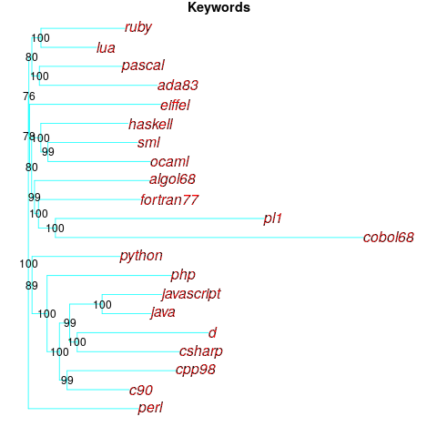
How confident should we be that this distance-based technique produced a robust result? For instance, would a small change to the set of keywords used by a particular language cause it to appear in a different branch of the tree?
The impact of small changes on the generated tree can be estimated using a bootstrap technique. The particular small-change algorithm used to estimate confidence levels for phylogenetic trees is not applicable for language keywords; genetic sequences contain multiple instances of four DNA bases, and can be sampled with replacement, while language keywords are a set of distinct items (i.e., cannot be sampled with replacement).
The bootstrap technique I used was: for each of the 21 languages in the data, was: add keywords to one language (the number added was 5% of the number of its existing keywords, randomly chosen from the set of all language keywords), calculate the distance matrix and build the corresponding tree, repeat 100 times. The 2,100 generated trees were then compared against the original tree, counting how many times each branch remained the same.
The numbers in the above plot show the percentage of generated trees where the same branching decision was made using the perturbed keyword data. The branching decisions all look very solid.
Can this keyword approach to language comparison be applied to all languages?
I think that most languages have some form of keywords. A few languages don’t use keywords (or reserved words), and there are some edge cases. Lisp doesn’t have any reserved words (they are functions), nor technically does Pl/1 in that the names of ‘word tokens’ can be defined as variables, and CHILL implementors have to choose between using Cobol or PL/1 syntax (giving CHILL two possible distinct sets of keywords).
To what extent are a language’s keywords representative of the language, compared to other languages?
One way to try and answer this question is to apply the distance/tree approach using other language traits; do the resulting trees have the same form as the keyword tree? The plot below shows the tree derived from the characters used to represent binary operators (code+data):
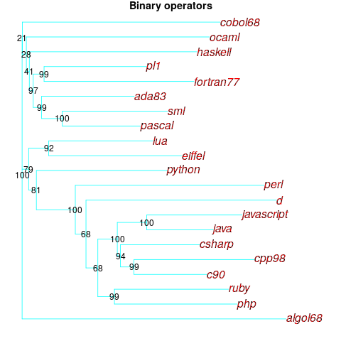
A few of the branching decisions look as-if they are likely to change, if there are changes to the keywords used by some languages, e.g., OCaml and Haskell.
Binary operators don’t just have a character representation, they can also have a precedence and associativity (neither are needed in languages whose expressions are written using prefix or postfix notation).
The plot below shows the tree derived from combining binary operator and the corresponding precedence information (the distance pairs for the two characteristics, for each language, were added together, with precedence given a weight of 20%; see code for details).
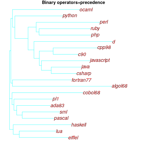
No bootstrap percentages appear because I could not come up with a simple technique for handling a combination of traits.
Are binary operators more representative of a language than its keywords? Would a combined keyword/binary operator tree would be more representative, or would more traits need to be included?
Does reducing language comparison to a single number produce something useful?
Languages contain a complex collection of interrelated components, and it might be more useful to compare their similarity by discrete components, e.g., expressions, literals, types (and implicit conversions).
What is the purpose of comparing languages?
If it is for promotional purposes, then a measurement based approach is probably out of place.
If the comparison has a source code orientation, weighting items by source code occurrence might produce a more applicable tree.
Sometimes one language is used as a reference, against which others are compared, e.g., C-like. How ‘C-like’ are other languages? Taking keywords as our reference-point, comparing languages based on just the keywords they have in common with C, the plot below is the resulting tree:
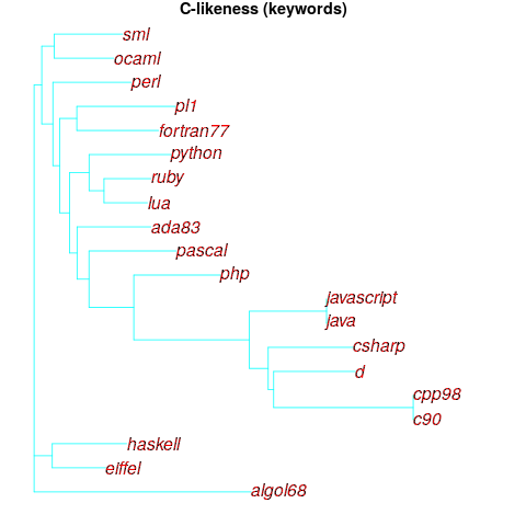
I had expected less branching, i.e., more languages having the same distance from C.
New languages can be supported by adding a language file containing the appropriate trait information. There is a Github repo, prog-lang-traits, send me a pull request to add your language file.
It’s also possible to add support for more language traits.
Ecology as a model for the software world
Changing two words in the Wikipedia description of Ecology gives “… the study of the relationships between software systems, including humans, and their physical environment”; where physical environment might be taken to include the hardware on which software runs and the hardware whose behavior it controls.
What do ecologists study? Wikipedia lists the following main areas; everything after the first sentence, in each bullet point, is my wording:
- Life processes, antifragility, interactions, and adaptations.
Software system life processes include its initial creation, devops, end-user training, and the sales and marketing process.
While antifragility is much talked about, it is something of a niche research topic. Those involved in the implementations of safety-critical systems seem to be the only people willing to invest the money needed to attempt to build antifragile software. Is N-version programming the poster child for antifragile system software?
Interaction with a widely used software system will have an influence on the path taken by cultures within associated microdomains. Users adapt their behavior to the affordance offered by a software system.
A successful software system (and even unsuccessful ones) will exist in multiple forms, i.e., there will be a product line. Software variability and product lines is an active research area.
- The movement of materials and energy through living communities.
Is money the primary unit of energy in software ecosystems? Developer time is needed to create software, which may be paid for or donated for free. Supporting a software system, or rather supporting the needs of the users of the software is often motivated by a salary, although a few do provide limited free support.
What is the energy that users of software provide? Money sits at the root; user attention sells product.
- The successional development of ecosystems (“… succession is the process of change in the species structure of an ecological community over time.”)
Before the Internet, monthly computing magazines used to run features on the changing landscape of the computer world. These days, we have blogs/podcasts telling us about the latest product release/update. The Ecosystems chapter of my software engineering book has sections on evolution and lifespan, but the material is sparse.
Over the longer term, this issue is the subject studied by historians of computing.
Moore’s law is probably the most famous computing example of succession.
- Cooperation, competition, and predation within and between species.
These issues are primarily discussed by those interested in the business side of software. Developers like to brag about how their language/editor/operating system/etc is better than the rest, but there is no substance to the discussion.
Governments have an interest in encouraging effective competition, and have enacted various antitrust laws.
- The abundance, biomass, and distribution of organisms in the context of the environment.
These are the issues where marketing departments invest in trying to shift the distribution in their company’s favour, and venture capitalists spend their time trying to spot an opportunity (and there is the clickbait of language popularity articles).
The abundance of tools/products, in an ecosystem, does not appear to deter people creating new variants (suggesting that perhaps ambition or dreams are the unit of energy for software ecosystems).
- Patterns of biodiversity and its effect on ecosystem processes.
Various kinds of diversity are important for biological systems, e.g., the mutual dependencies between different species in a food chain, and genetic diversity as a resource that provides a mechanism for species to adapt to changes in their environment.
It’s currently fashionable to be in favour of diversity. Diversity is so popular in ecology that a 2003 review listed 24 metrics for calculating it. I’m sure there are more now.
Diversity is not necessarily desired in software systems, e.g., the runtime behavior of source code should not depend on the compiler used (there are invariably edge cases where it does), and users want different editor command to be consistently similar.
Open source has helped to reduce diversity for some applications (by reducing the sales volume of a myriad of commercial offerings). However, the availability of source code significantly reduces the cost/time needed to create close variants. The 5,000+ different cryptocurrencies suggest that the associated software is diverse, but the rapid evolution of this ecosystem has driven developers to base their code on the source used to implement earlier currencies.
Governments encourage competitive commercial ecosystems because competition discourages companies charging high prices for their products, just because they can. Being competitive requires having products that differ from other vendors in a desirable way, which generates diversity.
NoEstimates panders to mismanagement and developer insecurity
Why do so few software development teams regularly attempt to estimate the duration of the feature/task/functionality they are going to implement?
Developers hate giving estimates; estimating is very hard and estimates are often inaccurate (at a minimum making the estimator feel uncomfortable and worse when management treats an estimate as a quotation). The future is uncertain and estimating provides guidance.
Managers tell me that the fear of losing good developers dissuades them from requiring teams to make estimates. Developers have told them that they would leave a company that required them to regularly make estimates.
For most of the last 70 years, demand for software developers has outstripped supply. Consequently, management has to pay a lot more attention to the views of software developers than the views of those employed in most other roles (at least if they want to keep the good developers, i.e., those who will have no problem finding another job).
It is not difficult for developers to get a general idea of how their salary, working conditions and practices compares with other developers in their field/geographic region. They know that estimating is not a common practice, and unless the economy is in recession, finding a new job that does not require estimation could be straight forward.
Management’s demands for estimates has led to the creation of various methods for calculating proxy estimate values, none of which using time as the unit of measure, e.g., Function points and Story points. These methods break the requirements down into smaller units, and subcomponents from these units are used to calculate a value, e.g., the Function point calculation includes items such as number of user inputs and outputs, and number of files.
How accurate are these proxy values, compared to time estimates?
As always, software engineering data is sparse. One analysis of 149 projects found that  , with the variance being similar to that found when time was estimated. An analysis of Function point calculation data found a high degree of consistency in the calculations made by different people (various Function point organizations have certification schemes that require some degree of proficiency to pass).
Managers don’t seem to be interested in comparing estimated Story points against estimated time, preferring instead to track the rate at which Story points are implemented, e.g., velocity, or burndown. There are tiny amounts of data comparing Story points with time and Function points.
The available evidence suggests a relationship connecting Function points to actual time, and that Function points have similar error bounds to time estimates; the lack of data means that Story points are currently just a source of technobabble and number porn for management power-points (send me Story point data to help change this situation).
Recent Comments