Archive
Studying the lifetime of Open source
A software system can be said to be dead when the information needed to run it ceases to be available.
Provided the necessary information is available, plus time/money, no software ever has to remain dead, hardware emulators can be created, support libraries can be created, and other necessary files cobbled together.
In the case of software as a service, the vendor may simply stop supplying the service; after which, in my experience, critical components of the internal service ecosystem soon disperse and are forgotten about.
Users like the software they use to be actively maintained (i.e., there are one or more developers currently working on the code). This preference is culturally driven, in that we are living through a period in which most in-use software systems are actively maintained.
Active maintenance is perceived as a signal that the software has some amount of popularity (i.e., used by other people), and is up-to-date (whatever that means, but might include supporting the latest features, or problem reports are being processed; neither of which need be true). Commercial users like actively maintained software because it enables the option of paying for any modifications they need to be made.
Software can be a zombie, i.e., neither dead or alive. Zombie software will continue to work for as long as the behavior of its external dependencies (e.g., libraries) remains sufficiently the same.
Active maintenance requires time/money. If active maintenance is required, then invest the time/money.
Open source software has become widely used. Is Open source software frequently maintained, or do projects inhabit some form of zombie state?
Researchers have investigated various aspects of the life cycle of open source projects, including: maintenance activity, pull acceptance/merging or abandoned, and turnover of core developers; also, projects in niche ecosystems have been investigated.
The commits/pull requests/issues, of circa 1K project repos with lots of stars, is data that can be automatically extracted and analysed in bulk. What is missing from the analysis is the context around the creation, development and apparent abandonment of these projects.
Application areas and development tools (e.g., editor, database, gui framework, communications, scientific, engineering) tend to have a few widely used programs, which continue to be actively worked on. Some people enjoy creating programs/apps, and will start development in an area where there are existing widely used programs, purely for the enjoyment or to scratch an itch; rarely with the intent of long term maintenance, even when their project attracts many other developers.
I suspect that much of the existing research is simply measuring the background fizz of look-alike programs coming and going.
A more realistic model of the lifecycle of Open source projects requires human information; the intent of the core developers, e.g., whether the project is intended to be long-term, primarily supported by commercial interests, abandoned for a successor project, or whether events got in the way of the great things planned.
Clustering source code within functions
The question of how best to cluster source code into functions is a perennial debate that has been ongoing since functions were first created.
Beginner programmers are told that clustering code into functions is good, for a variety of reasons (none of the claims are backed up by experimental evidence). Structuring code based on clustering the implementation of a single feature is a common recommendation; this rationale can be applied at both the function/method and file/class level.
The idea of an optimal function length (measured in statements) continues to appeal to developers/researchers, but lacks supporting evidence (despite a cottage industry of research papers). The observation that most reported fault appear in short functions is a consequence of most of a program’s code appearing in short functions.
I have had to deal with code that has not been clustered into functions. When microcomputers took off, some businessmen taught themselves to code, wrote software for their line of work and started selling it. If the software was a success, more functionality was needed, and the businessman (never encountered a woman doing this) struggled to keep on top of things. A common theme was a few thousand lines of unstructured code in one function in a single file (keeping everything in one file is also a trait of highly focus developers).
Adding structural bureaucracy (e.g., functions and multiple files) reduced the effort needed to maintain and enhance the code.
The problem with ‘born flat’ source is that the code for unrelated functionality is often intermixed, and global variables are freely used to communicate state. I have seen the same problems in structured function code, but instances are nowhere near as pervasive.
When implementing the same program, do different developers create functions implementing essentially the same functionality?
I am aware of two datasets relating to this question: 1) when implementing the same small specification (average length program 46.3 lines), a surprising number of variants (6,301) are created, 2) an experiment that asked developers to reintroduce functions into ‘flattened’ code.
The experiment (Alexey Braver’s MSc thesis) took an existing Python program, ‘flattened’ it by inlining functions (parameters were replaced by the corresponding call arguments), and asked subjects to “… partition it into functions in order to achieve what you consider to be a good design.”
The 23 rows in the plot below show the start/end (green/brown delimited by blue lines) of each function created by the 23 subjects; red shows code not within a function, and right axis is percentage of each subjects’ code contained in functions. Blue line shows original (currently plotted incorrectly; patched original code+data):
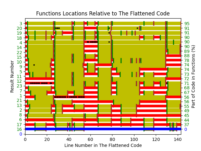
There are many possible reasons for the high level of agreement between subjects, including: 1) the particular example chosen, 2) the code was already well-structured, 3) subjects were explicitly asked to create functions, 4) the iterative process of discovering code that needs to be written did not occur, 5) no incentive to leave existing working code as-is.
Given that most source has a short and lonely existence, is too much time being spent bike-shedding function contents?
Given how often lower level design time happens at code implementation time, perhaps discussion of function contents ought to be viewed as more about thinking how things fit together and interact, than about each function in isolation.
Analyzing each function in isolation can create perverse incentives.
Printing press+widespread religious behavior: A theory
The book The Weirdest People in the World: How the West Became Psychologically Peculiar and Particularly Prosperous provides an explanation of the processes which weakened the existing social ties of family and tribe; however, the emergence of WEIRD people (Western, Educated, Industrialized, Rich and Democratic) required new social norms to spread and be accepted throughout society. A major technical innovation, in the form of the printing press, provided the means for mass communication of ideas and practices.
David High-Jones’ book Wyclif’s Dust: Western Cultures from the Printing Press to the Present describes the social consequences of what he calls book religion; a combination of deeply religious western societies and the ability of individuals to write and sell affordable books (made possible by the printing press). Religion+printing press created the conditions for what High-Jones calls a hothouse culture, a period from the 1600s to the end of the 1800s.
Around 1440 the printing press is invented and quickly spreads; around 5 million books were handwritten in the 1400s, about 80 million books were produced in the first 50 years of printing, and around a billion in the 1700s. During the 1500s the Protestant reformation happens; Protestant encouraged its followers to read the Bible, which creates a demand for printed Bibles and the need to be able to read (which increases literacy rates). In England, between 1480-1640, 40% of published books were religious.
The changes to society’s existing norms are wrought by cultural transmission, initially via middle class parents making use of edifying books to teach their children moral values and social skills, later Sunday schools took on this role, but also had to offer reading lessons to attract members. In the adult world, accepted norms were maintained by social enforcement. The impact on western societies was widespread because observant religious behavior was widespread.
The original intent, of those writing the religious books, was the creation of a god fearing society. In practice, a trust based society was created, where workers might be relied upon not to shirk their duties and businessmen to not renege on agreements.
In the beginning science, in the form of printed technical books, rarely made an appearance. In the 1700s the Enlightenment happens, and scientific books are discussed by small collections of disparate individuals. The industrial revolution happens, but the bulk of the demand is for trustworthy workers; technical and scientific know how remains a minority interest.
In Part I of the book, High-Jones weaves a reading and convincing narrative. Part II, 1900 to today, is a tale of the crumbling and breakdown of the social forces and incentives that creates the trust based society; while example are enumerated, no overarching theory is proposed (I skimmed this part).
Shopper estimates of the total value of items in their basket
Agile development processes break down the work that needs to be done into a collection of tasks (which may be called stories or some other name). A task, whose implementation time may be measured in hours or a few days, is itself composed of a collection of subtasks (which may in turn be composed of subsubtasks, and so on down).
When asked to estimate the time needed to implement a task, a developer may settle on a value by adding up estimates of the effort needed to implement the subtasks thought to be involved. If this process is performed in the mind of the developer (i.e., not by writing down a list of subtask estimates), the accuracy of the result may be affected by the characteristics of cognitive arithmetic.
Humans have two cognitive systems for processing quantities, the approximate number system (which has been found to be present in the brain of many creatures), and language. Researchers studying the approximate number system often ask subjects to estimate the number of dots in an image; I recently discovered studies of number processing that used language.
In a study by Benjamin Scheibehenne, 966 shoppers at the checkout counter in a grocery shop were asked to estimate the total value of the items in their shopping basket; a subset of 421 subjects were also asked to estimate the number of items in their basket (this subset were also asked if they used a shopping list). The actual price and number of items was obtained after checkout.
There are broad similarities between shopping basket estimation and estimating task implementation time, e.g., approximate idea of number of items and their cost. Does an analysis of the shopping data suggest ideas for patterns that might be present in software task estimate data?
The left plot below shows shopper estimated total item value against actual, with fitted regression line (red) and estimate==actual (grey); the right plot shows shopper estimated number of items in their basket against actual, with fitted regression line (red) and estimate==actual (grey) (code+data):
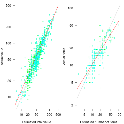
The model fitted to estimated total item value is:  , which differs from software task estimates/actuals in always underestimating over the range measured; the exponent value,
  , is at the upper range of those seen for software task estimates.
The model fitted to estimated number of items in the basket is:  . This pattern, of underestimating small values and overestimating large values is seen in software task estimation, but the exponent of
  is much smaller.
Including the estimated number of items in the shopping basket,  , in a model for total value produces a slightly better fitting model:
  , which explains 83% of the variance in the data (use of a shopping list had a relatively small impact).
The accuracy of a software task implementation estimate based on estimating its subtasks dependent on identifying all the subtasks, or having a good enough idea of the number of subtasks. The shopping basket study found a pattern of inaccuracies in estimates of the number of recently collected items, which has been seen before. However, adding to the Shopping model only reduced the unexplained variance by a few percent.
Would the impact of adding an estimate of the number of subtasks to models of software task estimates also only be a few percent? A question to add to the already long list of unknowns.
Like task estimates, round numbers were often given as estimate values; see code+data.
The same study also included a laboratory experiment, where subjects saw a sequence of 24 numbers, presented one at a time for 0.5 seconds each. At the end of the sequence, subjects were asked to type in their best estimate of the sum of the numbers seen (other studies asked subjects to type in the mean). Each subject saw 75 sequences, with feedback on the mean accuracy of their responses given after every 10 sequences. The numbers were described as the prices of items in a shopping basket. The values were drawn from a distribution that was either uniform, positively skewed, negatively skewed, unimodal, or bimodal. The sequential order of values was either increasing, decreasing, U-shaped, or inversely U-shaped.
Fitting a regression model to the lab data finds that the distribution used had very little impact on performance, and the sequence order had a small impact; see code+data.
Overview of broad US data on IT job hiring/firing and quitting
Software developers are employed by organizations and people change jobs, either voluntarily or not; every year a new batch of people join the workforce, e.g., new graduates. Governments track employment activities for a variety of reasons, e.g., tax collection, and monitoring labour supply and demand (for the purposes of planning).
The US Bureau of Labor Statistics’ publishes a monthly summary of their Job Openings and Labor Turnover Survey. What can be learned about software development employment from this data (description)?
The data starts in December 2000, with each row contains a monthly count of Job Openings, Hires, Quits, Layoffs and Discharges, and totals, along with one of 21 major non-farm industry codes or one of the 5 government codes (the counts are broken out by State). I’m guessing that software developers are assigned the Information code (i.e., 510000), but who is to say that some have not been classified with the code for, say, Construction or Education and health services. The Information code will cover a lot more than just software developers; I’m trading off broad IT coverage for monthly details on employment turnover (software developer specific information is available, but it comes without the turnover information). The Bureau of Labor Statistics make available a huge quantity of information, and understanding how it all fits together would probably require me to spend several months learning my way around (I have already spent a week or two over the years), so I’m sticking with a prebuilt dataset.
The plot below shows the aggregated monthly counts (i.e., all states) of Job Openings, Hires, Quits, Layoffs and Discharges for the Information industry code (code+data):
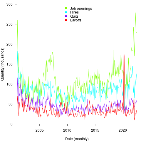
The general trend follows the ups and downs of the economy, there is a huge spike in layoffs in early 2020 (the start of COVID), and Job Openings often exceeding Hires (which I did not expect).
These counts have the form of a time-series, which leads to the questions about repeating patterns in the sequence of values? The plot below shows the autocorrelation of the four employment counts (code+data):
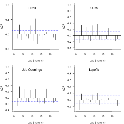
The spike in Hires at 12-months is too large to be just be new graduates entering the workforce; perhaps large IT employers have annual reviews for all employees at the same time every year, causing some people to quit and obtain new jobs (Quits has a slightly larger spike at 12-months). Why is there a regular 3-month cycle for Job Openings? The negative correlation in Layoffs at one & two months is explained by companies laying off a batch of workers one month, followed by layoffs in the following two months being lower than usual.
I don’t know much about employment practices, so I won’t speculate any more. Comments welcome.
Are there any interest cross-correlations between the pairs of time-series?
The plot below shows four pairs of cross correlations (code+data):
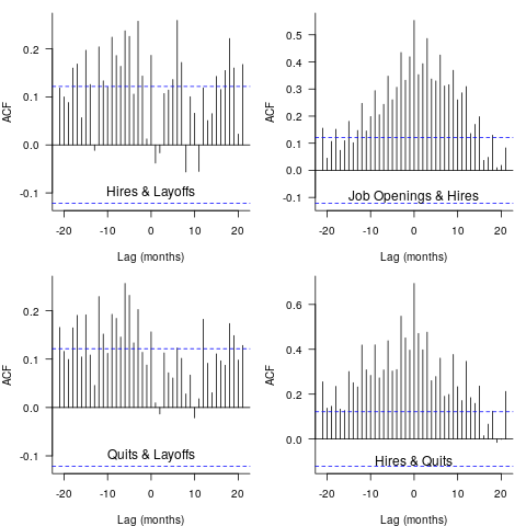
Hires & Layoffs shows a scattered pattern of Hires preceding Layoffs (to be expected), and the bottom left shows there is a pattern of Quits preceding Layoffs (are people searching for steadier employment when layoffs loom?). Top right shows a pattern of Job Openings following Hires (I’m clutching at straws for this; is Hires a proxy for Quits, the cross correlation of Job Openings & Quits does have Job Openings leading), the bottom right shows the pattern of Hires leading Quits.
Nothing in this analysis surprised me, but then it is rather basic and broad brush. These results are the start of an analysis of the IT employment ecosystem; one that probably won’t progress far because of a lack of data and interest on my part.
Optimal sizing of a product backlog
Developers working on the implementation of a software system will have a list of work that needs to be done, a to-do list, known as the product backlog in Agile.
The Agile development process differs from the Waterfall process in that the list of work items is intentionally incomplete when coding starts (discovery of new work items is an integral part of the Agile process). In a Waterfall process, it is intended that all work items are known before coding starts (as work progresses, new items are invariably discovered).
Complaints are sometimes expressed about the size of a team’s backlog, measured in number of items waiting to be implemented. Are these complaints just grumblings about the amount of work outstanding, or is there an economic cost that increases with the size of the backlog?
If the number of items in the backlog is too low, developers may be left twiddling their expensive thumbs because they have run out of work items to implement.
A parallel is sometimes drawn between items waiting to be implemented in a product backlog and hardware items in a manufacturer’s store waiting to be checked-out for the production line. Hardware occupies space on a shelf, a cost in that the manufacturer has to pay for the building to hold it; another cost is the interest on the money spent to purchase the items sitting in the store.
For over 100 years, people have been analyzing the problem of the optimum number of stock items to order, and at what stock level to place an order. The economic order quantity gives the optimum number of items to reorder,  (the derivation assumes that the average quantity in stock is
  ), it is given by:
 , where
  is the quantity consumed per year,
  is the fixed cost per order (e.g., cost of ordering, shipping and handling; not the actual cost of the goods),
  is the annual holding cost per item.
What is the likely range of these values for software?
- is around 1,000 per year for a team of ten’ish people working on multiple (related) projects; based on one dataset,
- is the cost associated with the time taken to gather the requirements, i.e., the items to add to the backlog. If we assume that the time taken to gather an item is less than the time taken to implement it (the estimated time taken to implement varies from hours to days), then the average should be less than an hour or two,
- : While the cost of a post-it note on a board, or an entry in an online issue tracking system, is effectively zero, there is the time cost of deciding which backlog items should be implemented next, or added to the next Sprint.
If the backlog starts with
 items, and it takes
  seconds to decide whether a given item should be implemented next, and
  is the fraction of items scanned before one is selected: the average decision time per item is:
 /2}*t") seconds. For example, if
seconds. For example, if  , pulling some numbers out of the air,
  , and
, and  , then
  , or 5.4 minutes.
The Scrum approach of selecting a subset of backlog items to completely implement in a Sprint has a much lower overhead than the one-at-a-time approach.
If we assume that  , then
  .
.
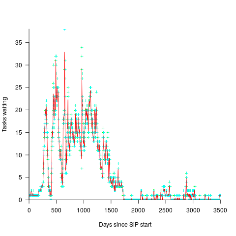
An ‘order’ for 45 work items might make sense when dealing with clients who have formal processes in place and are not able to be as proactive as an Agile developer might like, e.g., meetings have to be scheduled in advance, with minutes circulated for agreement.
In a more informal environment, with close client contacts, work items are more likely to trickle in or appear in small batches. The SiP dataset came from such an environment. The plot below shows the number of tasks in the backlog of the SiP dataset, for each day (blue/green) and seven-day rolling average (red) (code+data):
Career progression: an invisible issue in software development
Career progression is an important issue in the development of some software systems, but its impact is rarely discussed, let along researched. A common consequence of career progression is that a project looses a member of staff, e.g., they move to work on a different project, or leave the company. Hiring staff and promoting staff are related neglected research areas.
Understanding the initial and ongoing development of non-trivial software systems requires an understanding of the career progression, and expectations of progression, of the people working on the system.
Effectively working on a software system requires some amount of knowledge of how it operates, or is intended to operate. The loss of a person with working knowledge of a system reduces the rate at which a project can be further developed. It takes time to find a suitable replacement, and for that person’s knowledge of the behavior of the existing system to reach a workable level.
We know that most software is short-lived, but know almost nothing about the involvement-lifetime of those who work on software systems.
There has been some research studying the durations over which people have been involved with individual Open source projects. However, I don’t believe the findings from this research, because I think that non-paid involvement on an Open source project has very different duration and motivation characteristics than a paying job (there are also data cleaning issues around the same person using multiple email addresses, and people working in small groups with one person submitting code).
Detailed employment data, in bulk, has commercial value, and so is rarely freely available. It is possible to scrape data from the adverts of job websites, but this only provides information about the kinds of jobs available, not the people employed.
LinkedIn contains lots of detailed employment history, and the US courts have ruled that it is not illegal to scrape this data. It’s on my list of things to do, and I keep an eye out for others making such data available.
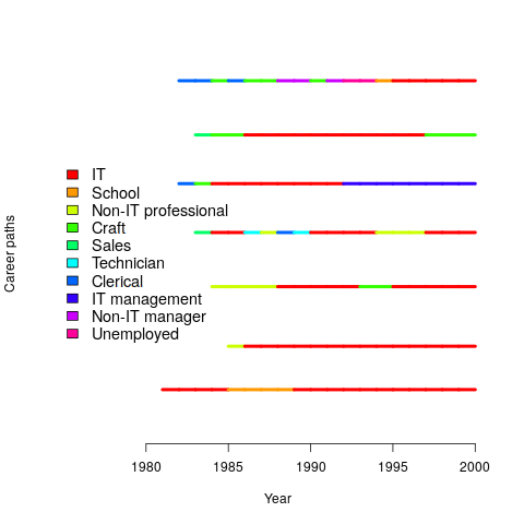
The National Longitudinal Survey of Youth has followed the lives of 10k+ people since 1979 (people were asked to detail their lives in periodic surveys). Using this data, Joseph, Boh, Ang, and Slaughter investigated the job categories within the career paths of 500 people who had worked in a technical IT role. The plot below shows the career paths of people who had spent at least five years working in an IT role (code+data):
Employment history provides an upper bound for the time that a person is likely to have worked on a project (being employed to work on an Open source project while, over time, working at multiple companies is an edge case).
A company may have employees simultaneously working on multiple projects, spending a percentage of their time on each. How big a resource impact is the loss of such a person? Were they simply the same kind of cog in multiple projects, or did they play an important synchronization role across projects? Details on all the projects a person worked on would help answer some questions.
Building a software system involves a lot more than writing the code. Technical managers working on high level, broad brush, issues. The project knowledge that technical managers have contributes to ongoing work, and the impact of loosing a technical manager is probably more of a longer term issue than loosing a coding-developer.
There are systems that are developed and maintained by essentially one person over many years. These get written about and celebrated, but are comparatively rare.
One of the more reliable ways of estimating developer productivity is to measure the impact of them leaving a project.
Programming Languages: History and Fundamentals
Programming Languages: History and Fundamentals by Jean E. Sammet is often cited in discussions of language history, but very rarely read (I appreciate that many oft cited books have not been read by those citing them, but age further reduces the likelihood that anybody has read this book; it was published in 1969). I read this book as an undergraduate, but did not think much of it. For around five years it has been on my list of books to buy, should a second-hand copy become available below £10 (I buy anything vaguely interesting below this price, with most ending up left on trains or the book table of coffee shops).
Thanks to Adam Gashlin the Internet Archive now contains a downloadable copy.
The list of 120 languages covered contains a handful of the 28 languages covered in an article from 1957. Sammet says that of the 120, 20 are already dead or on obsolete computers (i.e., it is unlikely that another compiler will be written), and that about 15 are widely used/implemented).
Today, the book is no longer a discussion of the recent past, but a window in to the Cambrian explosion of programming languages that happened in the 1960s (almost everything since then has been a variation on a theme); languages from the 1950s are also included.
How does the material appear to me from a 2022 vantage-point?
The organization of the book reminded me that programming languages were once categorized by application domain, i.e., scientific/engineering users, business users, and string & list processing (i.e., academic users). This division reflected the market segmentation for computer hardware (back then, personal computers were still in the realm of science fiction). Modern programming language books (e.g., Scott’s “Programming Language Pragmatics”) often organize material based on implementation details, e.g., lexical analysis, and scoping rules.
The overview of programming languages given in the first three chapters covers nearly all the basic issues that beginners are taught today, but the emphasis is different (plus typographical differences, such as keyword spelt ‘key word’).
Two major language constructs are missing: Dynamic storage allocation is not discussed: Wirth’s book Algorithms + Data Structures = Programs is seven years in the future, and Kernighan and Ritchie’s The C Programming Language nine years; Simula gets a paragraph, but no mention of the object-oriented concepts it introduced.
What is a programming language, and what are the distinguishing features that make some of them high-level programming languages?
These questions may sound pointless or obvious today, but people used to spend lots of time arguing over what was, or was not, a high-level language.
Sammet says: “… the first characteristic of a programming language is that the user can write a program without knowing much—if anything—about the physical characteristics of the machine on which the program is to be run.”, and goes on to infer: “… a major characteristic of a programming language is that there must be a reasonable potential of having a source program written in that language run on two computers with different machine codes without rewriting the source program. … In most programming languages, some—but often very little—rewriting of the source program is necessary.”
The reason that some rewriting of the source was likely to be needed is that there were often a lot of small variations between compilers for the same language. Compilers tended to be bespoke, i.e., the Fortran compiler for the X cpu running OS Y was written specifically for that combination. Retargetting an existing compiler to a new cpu or OS was much talked about, but it was more fun to write a new compiler (and anyway, support for new features was needed, and it was simpler to start from scratch; page 149 lists differences in Fortran compilers across IBM machines). It didn’t help that there was also a lot of variation in fundamental quantities such as word length, e.g., 16, 18, 20, 24, 32, 36, 40, 48, 60 bit words; see page 18 of Dictionary of Computer Languages.
Sammet makes the distinction: “One of the prime differences between assembly and higher level languages is that to date the latter do not have the capability of modifying themselves at execution time.”
Sammet then goes on to list the advantages and disadvantages of what she calls higher level languages. Most of the claimed advantages will be familiar to readers: “Ease of Learning”, “Ease of Coding and Understanding”, “Ease of Debugging”, and “Ease of Maintaining and Documenting”. The disadvantages included: “Time Required for Compiling” (the issue here is converting assembler source to object code is much faster than compiling a high-level language), “Inefficient Object Code” (the translation process was often a one-to-one mapping of what was written, e.g., little reuse of register contents), “Difficulties in Debugging Without Learning Machine Language” (symbolic debuggers are still in the future).
Sammet’s observation: “In spite of the fact that higher level languages have been with us for over 10 years, there has been relatively little quantitative or qualitative analysis of their advantages and disadvantages.” is still true 50 years later.
If you enjoy learning about lots of different languages, you will like this book. The discussion of specific languages contains copious examples, which for me brought things to life.
Sites such as the Internet Archive and Bitsavers make the book’s references accessible (there are a few I had not seen before), and offer readers a path to pre-Cambrian times.
Saul Rosen’s 1967 book “Programming Systems and Languages” is sometimes cited in discussions of programming language history. This book is a collection of papers that discuss a variety of languages and the operating systems that support them. Fewer languages are covered, but in more depth, along with lots of implementation details. Again, lots of interesting references.
Task backlog waiting times are power laws
Once it has been agreed to implement new functionality, how long do the associated tasks have to wait in the to-do queue?
An analysis of the SiP task data finds that waiting time has a power law distribution, i.e.,  , where
  is the number of tasks waiting a given amount of time; the LSST:DM Sprint/Story-point/Story has the same distribution. Is this a coincidence, or does task waiting time always have this form?
Queueing theory analyses the properties of systems involving the arrival of tasks, one or more queues, and limited implementation resources.
A basic result of queueing theory is that task waiting time has an exponential distribution, i.e., not a power law. What software task implementation behavior is sufficiently different from basic queueing theory to cause its waiting time to have a power law?
As always, my first line of attack was to find data from other domains, hopefully with an accompanying analysis modelling the behavior. It’s possible that my two samples are just way outside the norm.
Eventually I found an analysis of the letter writing response time of Darwin, Einstein and Freud (my email asking for the data has not yet received a reply). Somebody writes to a famous scientist (the scientist has to be famous enough for people to want to create a collection of their papers and letters), the scientist decides to add this letter to the pile (i.e., queue) of letters to reply to, eventually a reply is written. What is the distribution of waiting times for replies? Yes, it’s a power law, but with an exponent of -1.5, rather than -1.
The change made to the basic queueing model is to assign priorities to tasks, and then choose the task with the highest priority (rather than a random task, or the one that has been waiting the longest). Provided the queue never becomes empty (i.e., there are always waiting tasks), the waiting time is a power law with exponent -1.5; this behavior is independent of queue length and distribution of priorities (simulations confirm this behavior).
However, the exponent for my software data, and other data, is not -1.5, it is -1. A 2008 paper by Albert-László Barabási (detailed analysis) showed how a modification to the task selection process produces the desired exponent of -1. Each of the tasks currently in the queue is assigned a probability of selection, this probability is proportional to the priority of the corresponding task (i.e., the sum of the priorities/probabilities of all the tasks in the queue is assumed to be constant); task selection is weighted by this probability.
So we have a queueing model whose task waiting time is a power law with an exponent of -1. How well does this model map to software task selection behavior?
One apparent difference between the queueing model and waiting software tasks is that software tasks are assigned to a small number of priorities (e.g., Critical, Major, Minor), while each task in the model queue has a unique priority (otherwise a tie-break rule would have to be specified). In practice, I think that the developers involved do assign unique priorities to tasks.
Why wouldn’t a developer simply select what they consider to be the highest priority task to work on next?
Perhaps each developer does select what they consider to be the highest priority task, but different developers have different opinions about which task has the highest priority. The priority assigned to a task by different developers will have some probability distribution. If task priority assignment by developers is correlated, then the behavior is effectively the same as the queueing model, i.e., the probability component is supplied by different developers having different opinions and the correlation provides a clustering of priorities assigned to each task (i.e., not a uniform distribution).
If this mapping is correct, the task waiting time for a system implemented by one developer should have a power law exponent of -1.5, just like letter writing data.
The number of sprints that a story is assigned to, before being completely implemented, is a power law whose exponent varies around -3. An explanation of this behavior based on priority queues looks possible; we shall see…
The queueing models discussed above are a subset of the field known as bursty dynamics; see the review paper Bursty Human Dynamics for human behavior related aspects.
Patterns in the LSST:DM Sprint/Story-point/Story ‘done’ issues
Projects that use Scrum as their project management framework estimate tasks (known as a user story, or just story) in units of Story-points. A collection of User stories are grouped together to be implemented during a Sprint (a time-boxed interval, often lasting 2-weeks).
What are Story-points, and how do they map to time (in hours and minutes)? For this post, let’s ignore these questions, simply assuming that the people who assign a story-point value to a story have some mapping in their head.
What is the average number of story-points in a story, and how does this average vary across teams? What is the distribution of number of stories estimated per sprint, how many are actually implemented, and how does this vary across teams?
The data required to answer these questions has not been publicly available, or rather public data is not known to me. Until this week, I had only known of a few public Jira repos where story-points were given for at most a few hundred stories.
The LSST Corporation, a not-for-profit involved in astronomy and physics research, has a Data Management (DM) project. The Jira repo for this project contains 26,671 ‘Done’ issues (as of Aug 2022), of which 11,082 (41.5%) have assigned story-points; there have been 469 sprints, which involved 33% of the issues. The start/end implementation date/time for stories is mostly rather granular, and not fine enough to be used to attempt to correlate individual stories with hours. I found this repo, and a couple of others, via the paper Story points changes in agile iterative development, and downloaded all available issues.
What patterns are present in the story-point and sprint data?
Story points are commonly thought of as being integer valued, but 28% of the values are non-integer. If any developers are using the Fibonacci scale, there are not enough to have a noticeable impact. The plot below shows the number of stories estimated to involve a given number of story-points (black pluses are non-integer values, which have been rounded to fit the regression model). The green curved line is a fitted biexponential (sum of two exponentials), with the two straight lines being the two component exponentials (code+data):
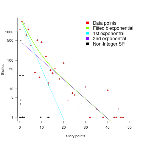
One exponential is dominant for stories assigned up to 10 story-points, and the second exponential for higher story-point values.
The development team decides to implement a story and allocates it to a sprint. A story may be reallocated to another sprint before the start of the original sprint, or after the sprint is finished when its implementation is incomplete or not yet started (the data does not allow for these cases to be distinguished). How many sprints is a story allocated to, before the story implementation is complete?
The plot below shows the number of stories allocated to a given number of sprints, with a fitted regression line of the form  (code+data):
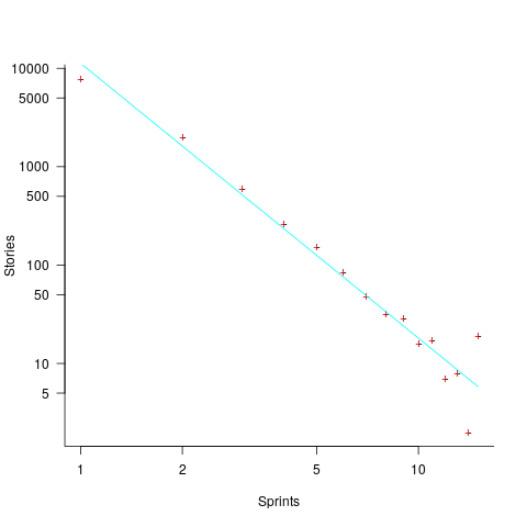
So around 14% of stories are allocated to two sprints, 5% to three and 2% to four.
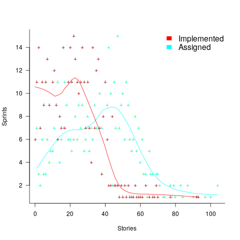
How many stories are assigned to a sprint? The plot below shows the number of sprints having a given number of stories assigned to them, and the number of sprints implementing a given number of stories; lines are fitted loess models (code+data):
Are the Story/Story-point/Sprint patterns found in the DM project likely to occur in other projects using Scrum?
I don’t know, but I hope so. Developing theories of software development processes requires that there be consistent patterns of behavior.
Not knowing what stories were assigned to a sprint at the start of the sprint, rather assigned earlier and then moved to another sprint, potentially undermines the sprint patterns. We will have to wait and see.
If anybody knows of any public Jira repos where a high percentage (say 40%) of the issues have been assigned story-points, please let me know (all the ones I know of on the Atlassian site contain a tiny percentage of story-points).
Recent Comments