Archive
Converting graphs in pdf files to csv format
Looking at a graph displayed as part of a pdf document is so tantalizing; I want that data as a csv!
One way to get the data is to email the author(s) and ask for it. I do this regularly and sometimes get the apologetic reply that the data is confidential. But I can see the data! Yes, but we only got permission to distribute the paper. I understand their position and would give the same reply myself; when given access to a company’s confidential data, explicit permission is often given about what can and cannot be made public with lists of numbers being on the cannot list.
The Portable Document Format was designed to be device independent, which means it contains a description of what to display rather than a bit-map of pixels (ok, it can contain a bit-map of pixels (e.g., a photograph) but this rather defeats the purpose of using pdf). It ought to be possible to automatically extract the data points from a graph and doing this has been on my list of things to do for a while.
I was mooching around the internals of a pdf last night when I spotted the line: /Producer (R 2.8.1); the authors had used R to generate the graphs and I could look at the R source code to figure out what was going on :-). I suspected that each line of the form: /F1 1 Tf 1 Tr 6.21 0 0 6.21 135.35 423.79 Tm (l) Tj 0 Tr was a description of a circle on the page and the function PDF_Circle in the file src/library/grDevices/src/devPS.c told me what the numbers meant; I was in business!
I also managed to match up other lines in the pdf file to the output produced by the functions PDF_Line and PDFSimpleText; it looked like the circles were followed by the axis tick marks and the label on each tick mark. Could things get any easier?
In suck-it-and-see projects like this it is best to use very familiar tools, this allows cognition to be focused on the task at hand. For me this meant using awk to match lines in pdf files and print out the required information.
Running the pdf through an awk script produced what looked like sensible x/y coordinates for circles on the page, the stop/start end-points of lines and text labels with their x/y coordinates. Now I needed to map the page x/y coordinates to within graph coordinate points.
After the circle coordinates in the output from the script were a series of descriptions of very short lines which looked like axis tick marks to me, especially since they were followed by coordinates of numbers that matched what appeared in the pdf graphs. This information is all that is needed to map from page coordinates to within graph coordinates. The graph I was interested in (figure 6) used logarithmic axis, so things were made a bit complicated by the need to perform a log transform.
Running the output (after some cut and pasting to removed stuff associated with other graphs in the pdf) from the first script through another awk script produced a csv file that could be fed into R’s plot to produce a graph that looked just like the original!
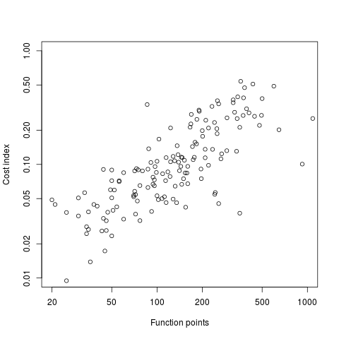
I would say it is possible to extract the data points from any graph, generated using R producing pdf or ps, contained within a pdf file.
The current scripts are very specific to the figure I was interested in, this is more to do with my rough and ready approach to solving the problem which makes assumptions about that is in the data; a more sophisticated version could handle common variations on the theme and with a bit of elbow grease point-and-click might be made to work.
It is probably also possible to extract data points in graphs produced by other tools, ‘all’ that is needed is information on the encoding used.
Extracting data from graphs generated to an image format such as png or jpg are going to need image processing software such as that used to extract data from images of tables.
Ordinary Least Squares is dead to me
Most books that discuss regression modeling start out and often finish with Ordinary Least Squares (OLS) as the technique to use; Generalized Linear ModelLeast Squares (GLMS) sometimes get a mention near the back. This is all well and good if the readers’ data has the characteristics required for OLS to be an applicable technique. A lot of data in the social sciences has these characteristics, or so I’m told; lots of statistics books are written for social science students, as a visit to a bookshop will confirm.
Software engineering datasets often range over several orders of magnitude or involve low value count data, not the kind of data that is ideally suited for analysis using OLS. For this kind of data GLMS is probably the correct technique to use (the difference in the curves fitted by both techniques is often small enough to be ignored for many practical problems, but the confidence bounds and p-values often differ in important ways).
The target audience for my book, Empirical Software Engineering with R, are working software developers who have better things to do that learn lots of statistics. However, there is no getting away from the fact that I am going to have to make extensive use of GLMS, which means having to teach readers about the differences between OLS and GLMS and under what circumstances OLS is applicable. What a pain.
Then I had a brainwave, or a moment of madness (time will tell). Why bother covering OLS? Why not tell readers to always use GLMS, or rather use the R function that implements it, glm. The default glm behavior is equivalent to lm (the R function that implements OLS); the calculation is not being done by hand but by a computer (i.e., who cares if it is more complicated).
Perhaps there is an easy way to explain this to software developers: glm is the generic template that can handle everything and lm is a specialized template that is tuned to handle certain kinds of data (the exact technical term will need tweaking for different languages).
There is one user interface issue, models built using glm do not come with an easy to understand goodness of fit number (lm has the R-squared value). AIC is good for comparing models but as a single (unbounded) number it is not that helpful for the uninitiated. Will the demand for R-squared be such that I will be forced for tell readers about lm? We will see.
How do I explain the fact that so many statistics books concentrate on OLS and often don’t mention GLMS? Hey, they are for social scientists, software engineering data requires more sophisticated techniques. I will have to be careful with this answer as it plays on software engineers’ somewhat jaded views of social scientists (some of whom have made very major contribution to CRAN).
All the software engineering data I have seen is small enough that the performance difference between glm/lm is not a problem. If performance is a real issue then readers will search the net and find out about lm; sorry guys but I want to minimise what the majority of readers need to know.
R now has its own shelf in Dillons
I was in Dillons, the one opposite University College London, at the start of the week and what did I spy there?

There is now a bookshelf devoted to R (right, second from top) in the programming languages section. The shelf would be a lot fuller if O’Reilly did not have a complete section devoted to their books.
A trolley of C/C++ books was waiting to refill the shelves near the door.

Being adjacent to a university means that programming language books make up a much larger percentage of software books.

And there is O’Reilly in the corner with two stacks of shelves.

And yes, this is a big bookshop, the front is a complete block; computing/mathematics/physics/chemistry/engineering/medicine are in the basement. You can buy skeletons and stethoscopes in the medical section a few rooms down from computing; a stethoscope is useful for locating strange noises in computer cases without having to open them.

Readers a bit younger than me probably know this shop as Waterstones.
I made a mistake, please don’t shoot me
The major difference between commercial/academic written software is the handling of user mistakes, or to be more exact what is considered to be a user mistake. In the commercial world the emphasis is on keeping the customer happy, which translates into trying hard to gracefully handle any ‘mistake’ the user makes. Academic software is generally written to solve a research problem and is often very unforgiving of users failing to keep to the undocumented straight and narrow; given the context this unforgiving behavior is understandable, but sometimes such software is released to an unsuspecting world.
The R archive of contributed packages, CRAN, is a good example of the academic approach to writing software. I am an active user of many packages in this archive and its contributors have my heart-felt thanks. But on a regular basis I make a mistake when calling a function in one of these packages, get shot in the foot and am not best pleased.
What makes the situation worse is that my mistakes are often so trivial and easy to fix (by both me or the package authors). My most common ‘mistake’ is passing an argument whose type is not handled by the function, e.g., passing a data-frame to diag (why do I have to convert the argument using as.matrix, when diag could spot my mistake and do the conversion for me instead of returning some horrible mess).
Commercial software can also be unforgiving of user mistakes; in fact early versions of a lot of commercial software is just as unfriendly as academic software. The difference is that the commercial managers will make it their business to ensure that developers fix the code to make it user friendly. Competition ensures that those who don’t listen to their users go out of business.
Updating code to gracefully handle user mistakes is often a chore and many developers hate having to do it, managers are needed to prod developers into doing the work. The only purpose for more than half of the code in a commercial product may be to handle user mistakes and the percentage can approach 90%.
A lot of Open Source software has significant commercial backing, e.g., Linux, Apache, Firefox and gcc/llvm, which means it is somebody’s job to make sure customer complaints are addressed.
What the R development team needs is more commercial backing (it appears to have very little, but I may be wrong). Then somebody can be hired to go through the popular packages to make then mistake friendly, feed the changes back to the original author and generally educate package developers about bullet proofing their code.
Amount of end-user usage of code in Firefox
How much end-user usage does the code in Firefox receive over time?
Short answer: The available data is very sparse and lots of hand waving is needed to concoct something.
The longer answer is below as another draft section from my book Empirical software engineering with R. As always, comments and pointers to more data welcome. R code and data here.
Suggestions for alternative methods of calculation also welcome.
Amount of end-user usage of code in Firefox
Source code that is never executed will not have any faults reported against it while code that is very frequently executed is more likely to have a fault reported against it than less frequently executed code.
The Firefox browser has been the subject of several fault related studies. The study by Massacci, Neuhaus and Nguyen is of interest here because it provides the information needed to attempt to build a fault model that takes account of the total amount of usage that code experiences from all end-users of a program. The data used by the study applies to 899 Mozilla Firefox-related Security Advisories (MFSA, a particular kind of fault), noting the earliest and latest versions of Firefox that exhibits each fault; six major releases (i.e., versions 1.0, 1.5, 2.0, 3.0, 3.5 and 3.6) were analysed; the amount of code in each version that originated in earlier versions was measured (see plot below).
Massacci et al make their raw data available under an agreement that does not permit your author to directly distribute it to readers;; the raw data for the following analysis was reverse engineered from the Massacci et al paper; or obtained from other sources.
The following analysis is an attempt to build a model of amount of Firefox code usage, by end-users, over time, i.e., number of lines of Firefox source code being executed per unit time summed over all end-users at a given moment in time. The intent is to couple this model with fault data, looking for a relationship of the form: an X% change in usage results in a Y% change in reported faults.
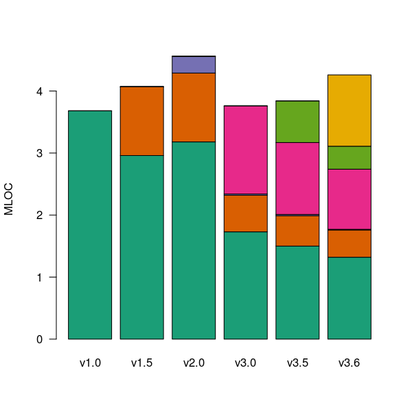
Figure 1. Amount of source (millions of lines) in each version, broken down by the version in which it first appears. Data from Massacci, Neuhaus and Nguyen <book Massacci_11>.
As expected, a large amount of code from previous versions appears in later versions.
Since we are interested in the relationship between end-user code usage and faults (MFSAs in this case) we are only interested in versions of Firefox that are actively maintained by Mozilla. Every version has a first official release date and an end-of-support date beyond which no faults reported against it are fixed; any usage of a version after the end-of-support date is not of interest in this analysis.
How many people are using each version of Firefox at any time?
A number of websites list information on Firefox market share over time (as a percentage of all browsers measured), but only two known to your author break this information down by Firefox version. Massacci et al used url[netmarketshare.com] for Firefox version market share (data going back to November 2007), but your author found it easier to obtain information from url[www.w3schools.com] (data going back to May 2007). The W3schools data is obtained from the log of visitors to their site, which will obviously be subject to fluctuations (of unknown magnitude).
For the period November 2004 to April 2007 the market share of each Firefox version was estimated as follows:
- total Firefox market share was based on that listed by url[marketshare.hitslink.com]
- during the period when only version 1.0 was available, its market share was assumed to be the total Firefox market share,
- the market share for versions 1.5 and 2.0 was assumed to follow the trend of growth and decline seen in later releases for which data is available. Numbers were concocted that followed the version trend and summed to the known total market share.
The plot below shows the market share of the six versions of Firefox between official release and end-of-support. Estimated values appear to the left of the vertical red line, values from measurements to the right. It can be seen that at its end-of-support date version 2.0 still had a significant market share.
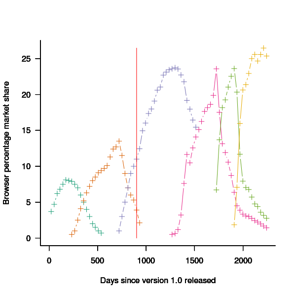
Figure 2. Market share of Firefox versions between official release and end-of-support. Data from url[www.w3schools.com].
The International Telecommunications Union publishers an estimate of the number of people per 100 head of population with Internet access for each year between 2003 and 2011 <book ITU_12>; the data is broken down by developed/developing countries and also by major world regions. Assuming that everybody who users the Internet uses a browser, this information can be combined with market share and human population data to estimate the number of Firefox users.
The ITU do not provide much information about how the usage figure is calculated or even which month of the year it applies to (since we are interested in change over time, knowing the month is not important and the start of the year is assumed). As the figure below shows the estimate over the period of interest can be accurately modeled by a straight line. A linear model was fitted to the data to predict usage between published estimates; over the period of interest the rate of growth in the Developed world has been almost twice as great as the rate in the whole world.
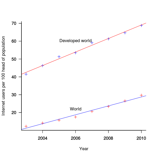
Figure 3. Number of people with Internet access per 100 head of population in the developed world and the whole world. Data from ITU <book <ITU_12>.
We are interested in relative change in total user population, and this can be obtained by multiplying the per-head of population value by the change in population (a 0.8% yearly growth is assumed for the developed world).
Possible significant factors for why the formula  might not accurately reflect the probability of a MFSA being reported include:
- the characteristics of people who started using the Internet in 2004 may be different from those who first started in 2010:
- there will be variation in the amount of time people spend browsing, does the distribution of time usage differ between early and late adopters?
- some people are more likely than others to report a fault (e.g., my mum is a late adopter and extremely unlikely to report a fault, whereas I might report a fault),
- there may be significant regional differences, e.g., European users vs. Chinese users. These differences include the Internet sites visited (the behavior of Firefox will depend on the content of the web page visited) and may affect their propensity to report a problem (e.g., do the cultural stereotypes of Chinese acceptance of authority mean they are unlikely to report a fault while those noisy Americans complain about everything?)
The end-user usage for code originally written for a particular version, at a point in time, is calculated as follows:
- number of lines of code originally written for a particular version that is contained within the code used to build a later version, or that particular version; call this the build version,
- times the market share of the build version,
- times the number of Internet users of the build version (users in the Developed world was used).
The plot below is an example using the source code originally written for Firefox version 1.0. The green points are the code usage for version 1.0 code executing in Firefox build version 1.0, the orange points the code usage for version 1.0 code executing in build version 1.5 and so on to the yellow points which is the code usage for version 1.0 code executing in build version 3.6. The black points are the sum over all build versions.
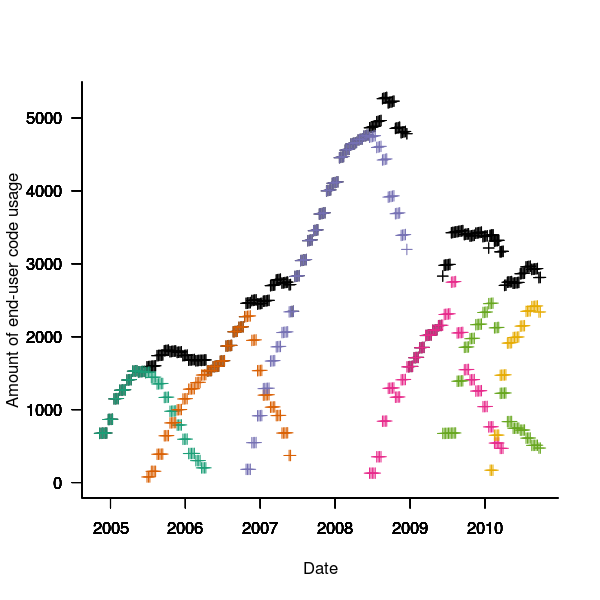
Figure 4. Amount of end-user usage of code originally written for Firefox version 1.0 by various other versions.
Much of the overall growth comes from growth in Internet usage, and in the early years there is also substantial growth in browser market share.
An analysis that attempts to connect Firefox usage with reported MFSAs will appear shortly (it would be surprising if fault report rate scaled linearly with end-user usage).
Unique bytes in a sliding window as a file content signature
I was at a workshop a few months ago where a speaker pointed out a useful technique for spotting whether a file contains compressed data, e.g., a virus hidden in a script by compressing it to look like a jumble of numbers. Compressed data contains a uniform distribution of byte values (after all, compression is achieved by reducing apparent information content), your mileage may vary between compression techniques. The thought struck me that it would only take a minute to knock up an R script to check out this claim (my use of R is starting to branch out into solving certain kinds of general coding problems) and here it is:
window_width=256  # if this is less than 256 divisor has to change in call to plot

plot_unique=function(filename)
{
t=readBin(filename, what="raw", n=1e7)

# Sliding the window over every point is too much overhead
cnt_points=seq(1, length(t)-window_width, 5)

u=sapply(cnt_points, function(X) length(unique(t[X:(X+window_width)])))
plot(u/256, type="l", xlab="Offset", ylab="Fraction Unique", las=1)

return(u)
}

dummy=plot_unique("http://shape-of-code.com/2013/05/17/preferential-attachment-applied-to-frequency-of-accessing-a-variable/")

dummy=plot_unique("http://www.shape-of-code.com/R_code/requirements.tgz") |
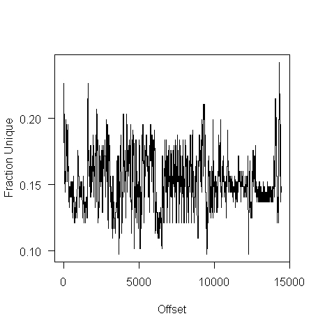
The unique bytes per window (256 bytes wide) of a HTML file has a mean around 15% (sd 2):
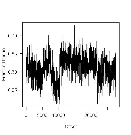
while for a tgz file the mean is 61% (sd 2.9):
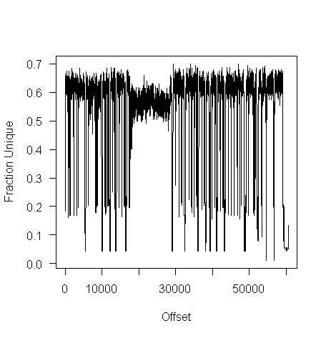
I don’t have any scripts containing a virus, but I do have a pdf containing lots of figures (are viruses hidden in pieces all all together?):
Do let me know if you find any interesting ‘unique byte’ signatures for file contents.
Prioritizing project stakeholders using social network metrics
Identifying project stakeholders and their requirements is a very important factor in the success of any project. Existing techniques tend to be very ad-hoc. In her PhD thesis Soo Ling Lim came up with a very interesting solution using social network analysis and what is more made her raw data available for download 🙂
I have analysed some of Soo Ling’s data below as another draft section from my book Empirical software engineering with R. As always comments and pointers to more data welcome. R code and data here.
A more detailed discussion and analysis is available in Soo Ling Lim’s thesis, which is very readable. Thanks to Soo Ling for answering my questions about her work.
Stakeholder roles and individuals
A stakeholder is a person who has an interest in what an application does. In a well organised development project the influential stakeholders are consulted before any contracts or budgets are agreed. Failure to identify the important stakeholders can result in missing or poorly prioritized requirements which can have a significant impact on the successful outcome of a project.
While many people might consider themselves to be stakeholders whose opinions should be considered, in practice the following groups are the most likely to have their opinions taken into account:
- people having an influence on project funding,
- customers, i.e., those people who are willing pay to use or obtain a copy of the application,
- domain experts, i.e., people with experience in the subject area who might suggest better ways to do something or problems to try and avoid,
- people who have influence over the success or failure over the actual implementation effort, e.g., software developers and business policy makers,
- end-users of the application (who on large projects are often far removed from those paying for it).
In the case of volunteer open source projects the only people having any influence are those willing to do the work. On open source projects made up of paid contributors and volunteers the situation is likely to be complicated.
Individuals have influence via the roles they have within the domain addressed by an application. For instance, the specification of a security card access system is of interest to the role of ‘being in charge of the library’ because the person holding that role needs to control access to various facilities provided within different parts of the library, while the role of ‘student representative’ might be interested in the privacy aspects of the information held by the application and the role of ‘criminal’ has an interest in how easy it is to circumvent the access control measures.
If an application is used by large numbers of people there are likely to be many stakeholders and roles, identifying all these and prioritizing them has, from experience, been found to be time consuming and difficult. Once stakeholders have been identified they then need to be persuaded to invest time learning about the proposed application and to provide their own views.
The RALIC study
A study by Lim <book Lim_10> was based on a University College London (UCL) project to combine different access control mechanisms into one, such as access to the library and fitness centre. The Replacement Access, Library and ID Card (RALIC) project had more than 60 stakeholders and 30,000 users, and has been deployed at UCL since 2007, two years before the study started. Lim created the StakeNet project with the aim of to identifying and prioritising stakeholders.
Because the RALIC project had been completed Lim had access to complete project documentation from start to finish. This documentation, along with interviews of those involved, were used to create what Lim called the Ground truth of project stakeholder role priority, stakeholder identification (85 people) and their rank within a role, requirements and their relative priorities; to quote Lim ‘The ground truth is the complete and prioritised list of stakeholders and requirements for the project obtained by analysing the stakeholders and requirements from the start of the project until after the system is deployed.’
The term salience is used to denote the level of a stakeholder’s influence.
Data
The data consists of three stakeholder related lists created as follows (all names have been made anonymous):
- the Ground truth list: derived from existing RALIC documentation. The following is an extract from this list (individual are ranked within each stakeholder role):
Role Rank,      Stakeholder Role,       Stakeholder Rank,       Stakeholder
1,      Security and Access Systems,    1,              Mike Dawson
1,      Security and Access Systems,    2,              Jason Ortiz
1,      Security and Access Systems,    3,              Nick Kyle
1,      Security and Access Systems,    4,              Paul Haywood
2,      Estates and Facilities Division,1,              Richard Fuller
- the Open list: starting from an initial list of 22 names and 28 stakeholder roles, four iterations of [Snowball sampling] resulted in a total of 61 responses containing 127 stakeholder names+priorities and 70 stakeholder roles,
- the Closed list: a list of 50 possible stakeholders was created from the RALIC project documentation plus names of other UCL staff added as noise. The people on this list were asked to indicated which of those names on the list they considered to be stakeholders and to assign them a salience between 1 and 10, they were also given the option to suggest names of possible stakeholders. This process generated a list containing 76 stakeholders names+priorities and 39 stakeholder roles.
The following is an extract from the last two stakeholder lists:
stakeholder stakeholder role salience David Ainsley Ian More 1 David Ainsley Rachna Kaplan 6 David Ainsley Kathleen Niche 4 David Ainsley Art Waller 1 David Carne Mark Wesley 4 David Carne Lis Hands 4 David Carne Vincent Matthew 4 Keith Lyon Michael Wondor 1 Keith Lyon Marilyn Gallo 1 Kerstin Michel Greg Beech 1 Kerstin Michel Mike Dawson 6 |
Is the data believable?
The data was gathered after the project was completed and as such it is likely to contain some degree of hindsight bias.
The data cleaning process is described in detail by Lim and looks to be thorough.
Predictions made in advance
Lim drew a parallel between the stakeholder prioritisation problem and the various techniques used to rank the nodes in social network analysis, e.g., the Page Rank algorithm. The hypothesis is that there is a strong correlation exists between the rank ordering of stakeholder roles in the Grounded truth list and the rank of stakeholder roles calculated using various social network metrics.
Applicable techniques
How might a list of people and the salience they assign to other people be converted to a single salience for each person? Lim proposed that social network metrics be used. A variety of techniques for calculating social network node centrality metrics have been proposed and some of these, including most used by Lim, are calculated in the following analysis.
Lim compared the Grounded truth ranking of stakeholder roles against the stakeholder role ranking created using the following network metrics:
- betweenness centrality: for a given node it is a count of the number of shortest paths from all nodes in a graph to all other nodes in that graph that pass through the given node; the value is sometimes normalised,
- closeness centrality: for a given node closeness is the inverse of farness, which is the sum of that node’s distances to all other nodes in the graph; the value is sometimes normalised,
- degree centrality: in-degree centrality is a count of the number of edges referring to a node, out-degree centrality is the number of edges that a node refers to; the value is sometimes normalised,
- load centrality: this is a variant of betweenness centrality based on the fraction of shortest paths through a given node. Support for load centrality is not available in the
igraphpackage and so is not used here, this functionality is available in thestatnetpackage, - pagerank: the famous algorithm proposed by Page and Brin <book Page_98> for ranking web pages.
Eigenvector centrality is another commonly used network metric and is included in this analysis.
Results
The igraph package includes functions for computing many of the common social network metrics. Reading data and generating a graph (the mathematical term for a social network) from it is particularly easy, in this case the graph.data.frame function is used to create a representation of its graph from the contents of a file read by read.csv.
The figure below plots Pagerank values for each node in the network created from the Open and Closed stakeholder salience ratings (Pagerank was chosen for this example because it had one of the strongest correlations with the Ground truth ranking). There is an obvious difference in the shape of the curves: the Open saliences (green) is fitted by the equation  (black line), while the Closed saliences (blue) is piecewise fitted by
  and
and  (red lines).
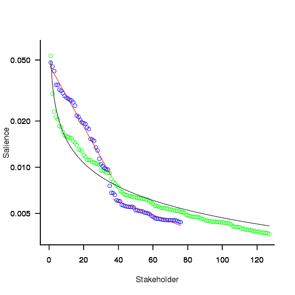
Figure 1. Plot of Pagerank of the stakeholder nodes in the network created from the Open (green) and Closed (blue) stakeholder responses (values for each have been sorted). See text for details of fitted curves.
To compare the ability of network centrality metrics to produce usable orderings of stakeholder roles a comparison has to be made against the Ground truth. The information in the Ground truth is a ranked list of stakeholder roles, not numeric values. The Stakeholder/centrality metric pairs need to be mapped to a ranked list of stakeholder roles. This mapping is achieved by associating a stakeholder role with each stakeholder name (this association was collected by Lim during the interview process), sorting stakeholder role/names by decreasing centrality metric and then ranking roles based on their first occurrence in the sorted list (see rexample[stakeholder]).
The Ground truth contains stakeholder roles not filled by any of the stakeholders in the Open or Closed data set, and vice versa. Before calculating role ranking correlation by roles not in both lists were removed.
The table below lists the Pearson correlation between the Ground truth ranking of stakeholder roles and for the ranking produced from calculating various network metrics from the Closed and Open stakeholder salience questionnaire data (when applied to ranks the Pearson correlation coefficient is equivalent to the Spearman rank correlation coefficient).
| betweenness | closeness | degree in | degree out | eigenvector | pagerank | |
|---|---|---|---|---|---|---|
|
Open
|
0.63
|
0.46
|
0.54
|
0.52
|
0.62
|
0.60
|
|
Weighted Open
|
0.66
|
0.49
|
0.62
|
0.50
|
0.68
|
0.67
|
|
Closed
|
0.51
|
0.53
|
0.67
|
0.60
|
0.69
|
0.71
|
|
Weighted Closed
|
0.50
|
0.50
|
0.63
|
0.54
|
0.68
|
0.72
|
The Open/Closed correlation calculation is based on a linear ranking. However, plotting Stakeholder salience, as in the plot above, shows a nonlinear distribution, with the some stakeholders having a lot more salience than less others. A correlation coefficient calculated by weighting the rankings may be more realistic. The “weighted” rows in the above are the correlations calculated using a weight based on the equations fitted in the Pagerank plot above; there is not a lot of difference.
Discussion
Network metrics are very new and applications making use of them still do so via a process of trial and error. For instance, the Pagerank algorithm was found to provide a good starting point for ranking web pages and many refinements have subsequently been added to the web ranking algorithms used by search engines.
When attempting to assign a priority to stakeholder roles and the people that fill them various network metric provide different ways of interpreting information about relationships between stakeholders. Lim’s work has shown that some network metrics can be used to produce ranks similar to those actually used (at least for one project).
One major factor not included in the above analysis is the financial contribution that each stakeholder role makes towards the implementation cost. Presumably those roles contributing a large percentage will want to be treated as having a higher priority than those contributing a smaller percentage.
The social network metrics calculated for stakeholder roles were only used to generate a ranking so that a comparison could be made against the ranked list available in the Ground truth. A rank ordering is a linear relationship between stakeholders; in real life differences in priority given to roles and stakeholders may not be linear. Perhaps the actual calculated network metric values are a better (often nonlinear) measure of relative difference, only experience will tell.
Summary of findings
Building a successful application is a very hard problem and being successful at it is something of a black art. There is nothing to say that a different Ground truth stakeholder role ranking would have lead to the RALIC project being just as successful. The relatively good correlation between the Ground truth ranking and the ranking created using some of the network metrics provides some confidence that these metrics might be of practical use.
Given that information on stakeholders’ rating of other stakeholders can be obtained relatively cheaply (Lim built a web site to collect this kind of information <book Lim_11>), for any large project a social network analysis appears to be a cost effect way of gathering and organizing information.
Never too experienced to make a basic mistake
I was one of the 170 or so people at the Data Science hackathon in London over the weekend. As always this was well run by Carlos and his team who kept us fed, watered and connected to the Internet.
One of the three challenges involved a dataset containing pairs of Twitter users, A and B, where one of the pair had been ranked, by a person, as more influential than the other (the data was provided by PeerIndex, an event sponsor). The dataset contained 22 attributes, 11 for each user of the pair, plus 0/1 to indicate who was most influential; there was a training dataset of 5.5K pairs to learn against and a test dataset to make predictions against. The data was not messy or even sparse, how hard could it be?
Talks had been organized for the morning and afternoon. While Microsoft (one of the event sponsors) told us about Azure and F#, I sat at the back trying out various machine learning packages. Yes, the technical evangelists told us, Linux as well as Windows instances were available in Azure, support was available for the usual big data languages (e.g., Python and R; the Microsoft people seemed to be much more familiar with Python) plus dot net (this was the first time I had heard the use of dot net proposed as a big data solution for the Cloud).
Some members of Team Outliers from previous hackathons (Jonny, Bob and me) formed a team and after the talks had finished the Microsoft people+partners sat at our table (probably because our age distribution was similar to theirs, i.e., at the opposite end of the range to most teams; some of the Microsoft people got very involved in trying to produce a solution to the visualization challenge).
Integrating F# with bigdata seems to involve providing an interface to R packages (this is done by interfacing to the packages installed on a local R installation) and getting the IDE to know about the names of columns contained in data that has been read. Since I think the world needs new general purpose programming languages as much as it needs holes in the head I won’t say any more.
When in challenge solving mode I was using cross-validation to check the models being built and scoring around 0.76 (AUC, the metric used by the organizers). Looking at the leader board later in the afternoon showed several teams scoring over 0.85, a big difference; what technique were they using to get such a big improvement?
A note: even when trained on data that uses 0/1 predictor values machine learners don’t produce models that return zero or one, many return values in the range 0..1 (some use other ranges) and the usual technique is treat all values greater than 0.5 as a 1 (or TRUE or ‘yes’, etc) and all other values as a 0 (or FALSE or ‘no’, etc). This (x > 0.5) test had to be done to cross validate models using the training data and I was using the same technique for the test data. With an hour to go in the 24 hour hackathon we found out (change from ‘I’ to ‘we’ to spread the mistake around) that the required test data output was a probability in the range 0..1, not just a 0/1 value; the example answer had this behavior and this requirement was explained in the bottom right of the submission page! How many times have I told others to carefully read the problem requirements? Thankfully everybody was tired and Jonny&Bob did not have the energy to throw me out of the window for leading them so badly astray.
Having AUC as the metric should have raised a red flag, this does not make much sense for a 0/1 answer; using AUC makes sense for PeerIndex because they will want to trade off recall/precision. Also, its a good idea to remove ones ego when asked the question: are lots of people doing something clever or are you doing something stupid?
While we are on the subject of doing the wrong thing, one of the top three teams gave an excellent example of why sales/marketing don’t like technical people talking to clients. Having just won a prize donated by Microsoft for an app using Azure, the team proceeded to give a demo and explain how they had done everything using Google services and made it appear within a browser frame as if it were hosted on Azure. A couple of us sitting at the back were debating whether Microsoft would jump in and disqualify them.
What did I learn that I did not already know this weekend? There are some R machine learning packages on CRAN that don’t include a predict function (there should be a research-only subsection on CRAN for packages like this) and some ranking algorithms need more than 6G of memory to process 5.5K pairs.
There seemed to be a lot more people using Python, compared to R. Perhaps having the sample solution in Python pushed the fence sitters that way. There also seemed to be more women present, but that may have been because there were more people at this event than previous ones and I am responding to absolute numbers rather than percentage.
Push hard on a problem here and it might just pop up over there
One thing I have noticed when reading other peoples’ R code is that their functions are often a lot longer than mine. Writing overly long functions is a common novice programmer mistake, but the code I am reading does not look like it is written by novices (based on the wide variety of base functions they are using, something a novice is unlikely to do, and by extrapolating my knowledge of novice behavior in other languages to R). I have a possible explanation for these longer functions, R users’ cultural belief that use of global variables is taboo.
Where did this belief originate? I think it can be traced back to the designers of R being paid up members of the functional programming movement of the early 80’s. This movement sought to mathematically prove programs correct but had to deal with the limitation that existing mathematical techniques were not really up to handling programs that contained states (e.g., variables that were assigned different values at different points in their execution). The solution was to invent a class of programming languages, functional languages, that did not provide any mechanisms for creating states (i.e., no global or local variables) and using such languages was touted as the solution to buggy code. The first half of the 80’s was full of computing PhD students implementing functional languages that had been designed by their supervisor, with the single application written by nearly all these languages being their own compiler.
Having to use a purely functional language to solve nontrivial problems proved to be mindbogglingly hard and support for local variables crept in and reading/writing files (which hold state) and of course global variables (but you must not use them because that would generate a side-effect; pointing to a use of a global variable in some postgrad’s code would result in agitated arm waving and references to a technique described in so-and-so’s paper which justified this particular use).
The functional world has moved on, or to be exact mathematical formalisms not exist that are capable of handling programs that have state. Modern users of functional languages don’t have any hangup about using global variables. The R community is something of a colonial outpost hanging on to views from a homeland of many years ago.
Isn’t the use of global variables recommended against in other languages? Yes and No. Many languages have different kinds of global variables, such as private and public (terms vary between languages); it is the use of public globals that may raise eyebrows, it may be ok to use them in certain ways but not others. The discussion in other languages revolves around higher level issues like information hiding and controlled access, ideas that R does not really have the language constructs to support (because R programs tend to be short there is rarely a need for such constructs).
Lets reformulate the question: “Is the use of global variables in R bad practice?”
The real question is: Given two programs, having identical external behavior, one that uses global variables and one that does not use global variables, which one will have the lowest economic cost? Economic cost here includes the time needed to figure out how to write the code and time to fix any bugs.
I am not aware of any empirical evidence, in any language, that answers this question (if you know of any please let me know). Any analysis of this question requires enumerating those problems where a solution involving a global variable might be thought to be worthwhile and comparing the global/nonglobal code; I know of a few snippets of such analysis in other languages.
Coming back to these long R functions, they often contain several for loops. Why are developers using for loops rather than the *ply functions? Is it because the *aply solution might require the use of a global variable, a cultural taboo that can be avoided by having everything in one function and using a for loop?
Next time somebody tells you that using global variables is bad practice you should ask for some evidence that backs that statement up.
I’m not saying that the use of global variables is good or bad, but that the issue is a complicated one. Enforcing a ‘no globals’ policy might just be moving the problem it was intended to solve to another place (inside long functions).
 distinct local variables have been accessed for reading
  times (
 ), will the next read access be from a previously unread local variable and if not what is the likelihood of choosing each of the distinct
  select a new variable to access,
  (where
  is the number of times the variable has previously been read from.
  read accesses to locally defined variables, how many variables will be read from only once, how many twice and so on (this is a static count extracted from the source code, not a dynamic count obtained by executing the function)?
 ; see rexample[local-use]):
 is the number of read accesses to a given variable and
  .
. select a new web page (in this case a new variable to access),
  select an existing web page (a variable that has previously been accessed in the function), select a variable with a probability proportional to the number of times it has previously been accessed (i.e., a variable that has four previous read accesses is twice as likely to be chosen as one that has had two previous accesses).
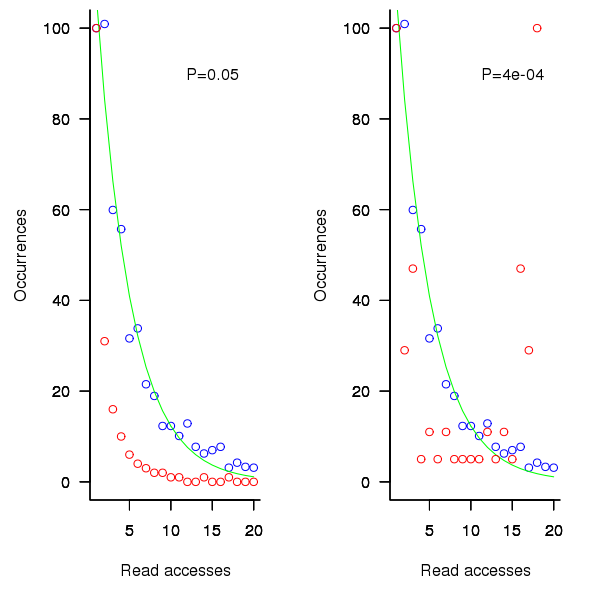
 (where
  so far) produces behavior that matches the data to the same degree as the exponential model.
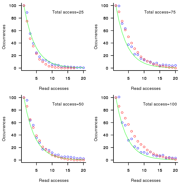
 select a variable that has previously been accessed in the function, select an existing variable with probability proportional to
  times as likely to be chosen as one that has had two previous accesses).
Recent Comments