Archive
Halstead/McCabe: a complicated formula for LOC
My experience is that people prefer to ignore the implications of Halstead’s metric and McCabe’s complexity metric being strongly correlated (non-linearly) with lines of code (LOC). The implications being that they have been deluding themselves and perhaps wasting time/money using Halstead/McCabe when they could just as well have used LOC.
If the purpose of collecting metrics is a requirement to tick a box, then it does not really matter which metrics are collected. The Halstead/McCabe metrics have a strong brand, so why not collect them.
Don’t make the mistake of thinking that Halstead/McCabe is more than a complicated way of calculating LOC. This can be shown by replacing Halstead/McCabe by the corresponding LOC value to find that it makes little difference to the value calculated.
Some metrics include the Halstead metrics and/or the McCabe metric as part of their calculation. The Maintainability Index is a metric calculated using Halstead’s volume, McCabe’s complexity and lines of code. Its equation is (see below for details):
-0.23*McCabe-16.2*ln(LOC)")
Replacing the Halstead/McCabe terms by one involving just LOC requires an appropriate mapping. Nearly all researchers assume a linear mapping, despite the overwhelming evidence that the mapping is non-linear.
Fitting regression models for HalsteadVolume vs LOC and McCabe vs LOC, using measurements of 730K methods from 47 Java projects (see below for data details), produces the coefficients for the equation needed to map each metric to LOC (previous analysis has found that a power law provides the best mapping; code+data). Substituting these equations in the Maintainability Index equation above, we get:
)-0.23*(0.45*LOC^{0.71})-16.2*ln(LOC)")
which simplifies to:
-0.1*LOC^{0.71}")
How does the value calculated using  compare with the corresponding
  value?
For 99.7% of methods, the relative error,  , for the 730K Java methods is less than 10%, and for 98.6% of methods the relative error is less than 5% (code+data).
Given the fuzzy nature of these metrics, 10% is essentially noise.
Looking at the relative contributions made by Halstead/McCabe/LOC to the value of the Maintainability Index, second equation above, the Halstead contribution is around a third the size of the LOC contribution and the McCabe contribution is at least an order of magnitude smaller.
Background on the Maintainability Index and the measured Java projects.
The Maintainability Index was introduced in the 1994 paper “Construction and Testing of Polynomials Predicting Software Maintainability” by Oman, and Hagemeister (270 citations; no online pdf), a 1992 paper by the same authors is often incorrectly cited (426 citations). The earlier 1992 paper identified 92 known maintainability attributes, along with 60 metrics for “… gauging software maintainability …” (extracted from 35 published papers).
This Maintainability Index equation was chosen from “Approximately 50 regression models were constructed and tested in our attempts to identify simple models that could be calculated from existing tools and still be generic enough to be applied to a wide range of software.” The data fitted came from eight suites of programs (average LOC 3,568 per suite), along “… with subjective engineering assessments of the quality and maintainability of each set of code.”
Yes, choosing from 50 regression models looks like overfitting, and by today’s standards 28.5K LOC is a tiny amount of source.
The data used is distributed with the paper Revisiting the Debate: Are Code Metrics Useful for Measuring Maintenance Effort? by Chowdhury, Holmes, Zaidman, and Kazman, which does a good job of outlining the many different definitions of maintenance and the inconsistent results from prediction models. However, the authors remain under the street light of project source code, i.e., they ignore the fact that many maintenance requests are driven by demand for new features.
The authors investigate the impact of normalizing Halstead/McCabe by LOC, but make the common mistake of assuming a linear relationship. They are surprised by the high correlation between post-‘normalised’ Halstead/McCabe and LOC. The correlation disappears when the appropriate non-linear normalization is used; see code+data.
A 2014 paper by Najm also maps the components of the Maintainability Index to LOC, but uses a linear mapping from the Halstead/McCabe terms to LOC, creating a equation whose behavior is noticeably different.
Half-life of Open source research software projects
The evidence for applications having a half-life continues to spread across domains. The first published data covered IBM mainframe applications up to 1992 (half-life of at least 5-years), and was mostly ignored. Then, the data collected by Killed by Google up to 2018, showed a half-life of at least 3-years for Google apps. More recently, the data collected by Killed by Microsoft up to 2025, showed a half-life of at least 7-years for Microsoft apps (perhaps reflecting the maturity of the company’s product line).
The half-life of source code, independent of the lifetime of the application it implements, is a separate topic.
Scientific software created to support researchers is an ecosystem whose incentives and means of production can be very different from commercial software. Does researcher oriented software die when the grant money runs out, or the researcher moves on to the next fashionable topic, or does it live on as the field expands?
The paper Scientific Open-Source Software Is Less Likely to Become Abandoned Than One Might Think! Lessons from Curating a Catalog of Maintained Scientific Software by Thakur, Milewicz, Jahanshahi, Paganini, Vasilescu, and Mockus analysed 14,418 scientific software systems written in Python (53%), C/C++ (25%), R (12%), Java (8%) or Fortran (2%). The first half of the paper describes how World of Code‘s 209 million repos were filtered down to 350,308 projects containing README files, these READMEs were processed by LLMs to extract information and further filter out projects.
The authors collected the usual information about each Open source project, e.g., number of core developers, number of commits, programming language, etc. They also collected information about the research domain, e.g., scientific field (biology, chemistry, mathematics, etc.), funding, academic/government associations, etc. A Cox proportional hazards model was fitted to this data, with project lifetime being the response variable. A project was deemed to have been abandoned when no changes had been made to the code for at least six consecutive months (we can argue over whether this is long enough).
Including all the different factors created a Cox model that did a good job of explaining the variance in project survival rate. No one factor dominated, and there was a lot of overlap in the confidence bounds of the components of each factor, e.g., different research domains. I have always said that programming language has no impact on project lifetime; the language factor of the fitted model was not statistically significant (two of the languages just sneaked in under the 5% bar), which can be interpreted as being consistent with my opinion.
Each project was categorised as one of: Scientific Domain-specific code (73.5%), Scientific infrastructure (16.5%), or Publication-Specific code (10%). The plot below shows the Kaplan-Meier survival curve for these three categories (note: y-axis is logarithmic), with faint grey lines showing a fitted exponential for each survival curve (only 3% of projects are abandoned in the first year, and the exponential fits are to the data after the first year; code+data):
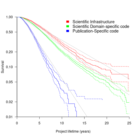
Readers familiar with academic publishing will not be surprised that projects associated with published papers have the lowest survival rate (half-life just over 2-years). Infrastructure projects are likely to be depended on by many people, who all have an interest in them surviving (half-life around 6-years). The Domain-specific half-life is around 4.5-years.
The results of this study show software systems in various research ecosystems having a range of half-lives in the same range as three major commercial software ecosystems.
Unfortunately, my experience of discussing application half-life with developers is that they believe in an imagined future where software never dies. That is, they are unwilling to consider a world where software has a high probability of being abandoned, because it requires that they consider the return on investment before spending time polishing their code.
Positive and negative descriptions of numeric data
Effective human communication is based on the cooperative principle, i.e., listeners and speakers act cooperatively and mutually accept one another to be understood in a particular way. However, when seeking to present a particular point of view, speakers may prefer to be economical with the truth.
To attract citations and funding, researchers sell their work via the papers they publish (or blogs they write), and what they write is not subject to the Advertising Standards Authority rule that “no marketing communication should mislead, or be likely to mislead, by inaccuracy, ambiguity, exaggeration, omission or otherwise” (my default example).
When people are being economical with the truth, when reporting numeric information, are certain phrases or words more likely to be used?
The paper: Strategic use of English quantifiers in the reporting of quantitative information by Silva, Lorson, Franke, Cummins and Winter, suggests some possibilities.
In an experiment, subjects saw the exam results of five fictitious students and had to describe the results in either a positive or negative way. They were given a fixed sentence and had to fill in the gaps by selecting one of the listed words; as in the following:
             all                      all
             most                     most                  right
In this exam .... of the students got .... of the questions .....
             some                     some                  wrong
none none |
If you were shown exam results with 2 out of 5 students failing 80% of questions and the other 3 out of 5 passing 80% of questions, what positive description would you use, and what negative description would you use?
The 60 subjects each saw 20 different sets of exam results for five fictitious students. The selection of positive/negative description was random for each question/subject.
The results found that when asked to give a positive description, most responses focused on questions that were right, and when asked to give a negative description, most responses focused on questions that were wrong
How many questions need to be answered correctly before most can be said to be correct? One study found that at least 50% is needed.
“3 out of 5 passing 80%” could be described as “… most of the students got most of the questions right.”, and “2 out of 5 students failing 80%” could be described as “… some of the students got most of the questions wrong.”
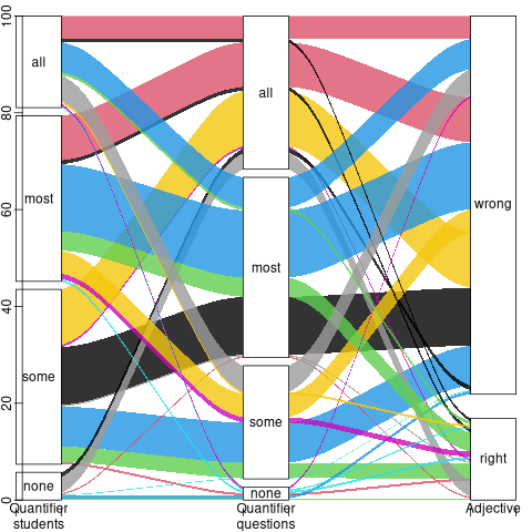
The authors fitted a Bayesian linear mixed effect models, which showed a somewhat complicated collection of connections between quantifier use and exam results. The plots below provide a visual comparison of the combination of quantifier use for positive (upper) and negative (lower) descriptions.
The alluvial plot below shows the percentage flow, for Positive descriptions, of each selected quantifier through student and question, and then adjective (code+data):

For the same distribution of exam results, the alluvial plot below shows the percentage flow, for Negative descriptions, of each selected quantifier through student and question, and then adjective (code+date):
Other adjectives could be used to describe the results (e.g., few, several, many, not many, not all), and we will have to wait for the follow-up research to this 2024 paper.
Predicted impact of LLM use on developer ecosystems
LLMs are not going to replace developers. Next token prediction is not the path to human intelligence. LLMs provide a convenient excuse for companies not hiring or laying off developers to say that the decision is driven by LLMs, rather than admit that their business is not doing so well
Once the hype has evaporated, what impact will LLMs have on software ecosystems?
The size and complexity of software systems is limited by the human cognitive resources available for its production. LLMs provide a means to reduce the human cognitive effort needed to produce a given amount of software.
Using LLMs enables more software to be created within a given budget, or the same amount of software created with a smaller budget (either through the use of cheaper, and presumably less capable, developers, or consuming less time of more capable developers).
Given the extent to which companies compete by adding more features to their applications, I expect the common case to be that applications contain more software and budgets remain unchanged. In a Red Queen market, companies want to be perceived as supporting the latest thing, and the marketing department needs something to talk about.
Reducing the effort needed to create new features means a reduction in the delay between a company introducing a new feature that becomes popular, and the competition copying it.
LLMs will enable software systems to be created that would not have been created without them, because of timescales, funding, or lack of developer expertise.
I think that LLMs will have a large impact on the use of programming languages.
The quantity of training data (e.g., source code) has an impact on the quality of LLM output. The less widely used languages will have less training data. The table below lists the gigabytes of source code in 30 languages contained in various LLM training datasets (for details see The Stack: 3 TB of permissively licensed source code by Kocetkov et al.):
Language TheStack CodeParrot AlphaCode CodeGen PolyCoder HTML 746.33 118.12 JavaScript 486.2 87.82 88 24.7 22 Java 271.43 107.7 113.8 120.3 41 C 222.88 183.83 48.9 55 C++ 192.84 87.73 290.5 69.9 52 Python 190.73 52.03 54.3 55.9 16 PHP 183.19 61.41 64 13 Markdown 164.61 23.09 CSS 145.33 22.67 TypeScript 131.46 24.59 24.9 9.2 C# 128.37 36.83 38.4 21 GO 118.37 19.28 19.8 21.4 15 Rust 40.35 2.68 2.8 3.5 Ruby 23.82 10.95 11.6 4.1 SQL 18.15 5.67 Scala 14.87 3.87 4.1 1.8 Shell 8.69 3.01 Haskell 6.95 1.85 Lua 6.58 2.81 2.9 Perl 5.5 4.7 Makefile 5.09 2.92 TeX 4.65 2.15 PowerShell 3.37 0.69 FORTRAN 3.1 1.62 Julia 3.09 0.29 VisualBasic 2.73 1.91 Assembly 2.36 0.78 CMake 1.96 0.54 Dockerfile 1.95 0.71 Batchfile 1 0.7 Total 3135.95 872.95 715.1 314.1 253.6 |
The major companies building LLMs probably have a lot more source code (as of July 2023, the Software Heritage had over  unique source code files); this table gives some idea of the relative quantities available for different languages, subject to recency bias. At the moment, companies appear to be training using everything they can get their hands on. Would LLM performance on the widely used languages improve if source code for most of the 682 languages listed on Wikipedia was not included in their training data?
Traditionally, developers have had to spend a lot of time learning the technical details about how language constructs interact. For the first few languages, acquiring fluency usually takes several years.
It’s possible that LLMs will remove the need for developers to know much about the details of the language they are using, e.g., they will define variables to have the appropriate type and suggest possible options when type mismatches occur.
Removing the fluff of software development (i.e., writing the code) means that developers can invest more cognitive resources in understanding what functionality is required, and making sure that all the details are handled.
Removing a lot of the sunk cost of language learning removes the only moat that some developers have. Job adverts could stop requiring skills with particular programming languages.
Little is currently known about developer career progression, which means it’s not possible to say anything about how it might change.
Since they were first created, programming languages have fascinated developers. They are the fashion icon of software development, with youngsters wanting to program in the latest language, or at least not use the languages used by their parents. If developers don’t invest in learning language details, they have nothing language related to discuss with other developers. Programming languages will cease to be a fashion icon (cpus used to be a fashion icon, until developers did not need to know details about them, such as available registers and unique instructions). Zig could be the last language to become fashionable.
I don’t expect the usage of existing language features to change. LLMs mimic the characteristics of the code they were trained on.
When new constructs are added to a popular language, it can take years before they start to be widely used by developers. LLMs will not use language constructs that don’t appear in their training data, and if developers are relying on LLMs to select the appropriate language construct, then new language constructs will never get used.
By 2035 things should have had time to settle down and for the new patterns of developer behavior to be apparent.
Impact of developer uncertainty on estimating probabilities
For over 50 years, it has been known that people tend to overestimate the likelihood of uncommon events/items occurring, and underestimate the likelihood of common events/items. This behavior has replicated in many experiments and is sometimes listed as a so-called cognitive bias.
Cognitive bias has become the term used to describe the situation where the human response to a problem (in an experiment) fails to match the response produced by the mathematical model that researchers believe produces the best output for this kind of problem. The possibility that the mathematical models do not reflect the reality of the contexts in which people have to solve the problems (outside of psychology experiments), goes against the grain of the idealised world in which many researchers work.
When models take into account the messiness of the real world, the responses are a closer match to the patterns seen in human responses, without requiring any biases.
The 2014 paper Surprisingly Rational: Probability theory plus noise explains biases in judgment by F. Costello and P. Watts (shorter paper), showed that including noise in a probability estimation model produces behavior that follows the human behavior patterns seen in practice.
If a developer is asked to estimate the probability that a particular event,  , occurs, they may not have all the information needed to make an accurate estimate. They may fail to take into account some s, and incorrectly include other kinds of events as being s. This noise,
  , introduces a pattern into the developer estimate:
*P_E + N*(1-P_E)=(1-2N)*P_E+N")
where:  is the developer’s estimated probability of event occurring,
  is the actual probability of the event, and is the probability that noise produces an incorrect classification of an event as
  or (for simplicity, the impact of noise is assumed to be the same for both cases).
The plot below shows actual event probability against developer estimated probability for various values of , with a red line showing that at  , the developer estimate matches reality (code):

The effect of noise is to increase probability estimates for events whose actually probability is less than 0.5, and to decrease the probability when the actual is greater than 0.5. All estimates move towards 0.5.
What other estimation behaviors does this noise model predict?
If there are two events, say  and
and  , then the noise model (and probability theory) specifies that the following relationship holds:
+P(B) == P(A & B)+P(A delim{|}{B}{})")
where: ") denotes the probability of its argument.
denotes the probability of its argument.
The experimental results show that this relationship does hold, i.e., the noise model is consistent with the experiment results.
This noise model can be used to explain the conjunction fallacy, i.e., Tversky & Kahneman’s famous 1970s “Lindy is a bank teller” experiment.
What predictions does the noise model make about the estimated probability of experiencing  (
( ) occurrences of the event in a sequence of
  assorted events (the previous analysis deals with the case
  )?
)?
An estimation model that takes account of noise gives the equation:

where:  is the developer’s estimated probability of experiencing s in a sequence of length , and
  is the actual probability of there being .
The plot below shows actual event probability against developer estimated probability for various values of , with a red line showing that at , the developer estimate matches reality (code):

This predicted behavior, which is the opposite of the case where , follows the same pattern seen in experiments, i.e., actual probabilities less than 0.5 are decreased (towards zero), while actual probabilities greater than 0.5 are increased (towards one).
There have been replications and further analysis of the predictions made by this model, along with alternative models that incorporate noise.
To summarise:
When estimating the probability of a single event/item occurring, noise/uncertainty will cause the estimated probability to be closer to 50/50 than the actual probability.
When estimating the probability of multiple events/items occurring, noise/uncertainty will cause the estimated probability to move towards the extremes, i.e., zero and one.
Recent Comments