Archive
Modeling the distribution of method sizes
The number of lines of code in a method/function follows the same pattern in the three languages for which I have measurements: C, Java, Pharo (derived from Smalltalk-80).
The number of methods containing a given number of lines is a power law, with an exponent of 2.8 for C, 2.7 for Java and 2.6 for Pharo.
This behavior does not appear to be consistent with a simplistic model of method growth, in lines of code, based on the following three kinds of steps over a 2-D lattice: moving right with probability  , moving up and to the right with probability
  , and moving down and to the right with probability
  . The start of an
 if or for statement are examples of coding constructs that produce a step followed by a step at the end of the statement; steps are any non-compound statement. The image below shows the distinct paths for a method containing four statements:

For this model, if  the probability of returning to the origin after taking
  is a complicated expression with an exponentially decaying tail, and the case
  is a well studied problem in 1-D random walks (the probability of returning to the origin after taking steps is
  approx n^{-1.5}") ).
).
Possible changes to this model to more closely align its behavior with source statement production include:
- include terms for the correlation between statements, e.g., assigning to a local variable implies a later statement that reads from that variable,
- include context terms in the up/down probabilities, e.g., nesting level.
Measuring statement correlation requires handling lots of special cases, while measurements of up/down steps is easily obtained.
How can / probabilities be written such that step length has a power law with an exponent greater than two?
ChatGPT 5 told me that the Langevin equation and Fokker–Planck equation could be used to derive probabilities that produced a power law exponent greater than two. I had no idea had they might be used, so I asked ChatGPT, Grok, Deepseek and Kimi to suggest possible equations for the / probabilities.
The physics model corresponding to this code related problem involves the trajectories of particles at the bottom of a well, with the steepness of the wall varying with height. This model is widely studied in physics, where it is known as a potential well.
Reaching a possible solution involved refining the questions I asked, following suggestions that turned out to be hallucinations, and trying to work out what a realistic solution might look like.
One ChatGPT suggestion that initially looked promising used a Metropolis–Hastings approach, and a logarithmic potential well. However, it eventually dawned on me that ^a") , where
, where  is nesting level, and
  some constant, is unlikely to be realistic (I expect the probability of stepping up to decrease with nesting level).
Kimi proposed a model based on what it called algebraic divergence:
=r/{z(y)},U(y)={u_0y^{1-2/{alpha}}}/{z(y)}, D(y)={d_0y^{1-2/{alpha}}}/{z(y)}")
where: ") normalises the probabilities to equal one,
normalises the probabilities to equal one, =r+u_0y^{1-2/alpha}+d_0y^{1-2/alpha}") ,
,  is the up probability at nesting 0,
  is the down probability at nesting 0, and
  is the desired power law exponent (e.g., 2.8).
For C,  , giving
 =r/{z(y)},U(y)={u_0y^{0.29}}/{z(y)}, D(y)={d_0y^{0.29}}/{z(y)}")
The average length of a method, in LOC, is given by:
![E[LOC]={alpha r}/{2(d_0-u_0)}+O(e^{lambda}-1)](https://shape-of-code.com/wp-content/plugins/wpmathpub/phpmathpublisher/img/math_969.5_ffcacf0bb8190096d4d17fb475c0a290.png "E[LOC]={alpha r}/{2(d_0-u_0)}+O(e^{lambda}-1)") , where:
, where: }/{d_0+u_0}")
For C, the mean function length is 26.4 lines, and the values of  , , and need to be chosen subject to the constraint
  .
.
Combining the normalization factor with the requirement  , shows that as increases,
 ") slowly decreases and
slowly decreases and ") slowly increases.
slowly increases.
One way to judge how closely a model matches reality is to use it to make predictions about behavior patterns that were not used to create the model. The behavior patterns used to build this model were: function/method length is a power law with exponent greater than 2. The mean length, ![E[LOC]](https://shape-of-code.com/wp-content/plugins/wpmathpub/phpmathpublisher/img/math_981.5_0ac27fa76bd7c6e393f3497c9f30db7e.png "E[LOC]") , is a tuneable parameter.
, is a tuneable parameter.
Ideally a model works across many languages, but to start, given the ease of measuring C source (using Coccinelle), this one language will be the focus.
I need to think of measurable source code patterns that are not an immediate consequence of the power law pattern used to create the model. Suggestions welcome.
It’s possible that the impact of factors not included in this model (e.g., statement correlation) is large enough to hide any nesting related patterns that are there. While different kinds of compound statements (e.g., if vs. for) may have different step probabilities, in C, and I suspect other languages, if-statement use dominates (Table 1713.1: if 16%, for 4.6% while 2.1%, non-compound statements 66%).
Early research on economies of scale for computer systems
Before microprocessor cost/performance wiped out (in the early 1990s) other cpu platforms (e.g., mainframes and minis), people argued that computer hardware benefited from economies of scale.
The claimed benefit was more bang for the buck, i.e., more compute for less money.
Checking this claim requires treating pre-microprocessor computer systems and the later microprocessor-based systems as two separate cases, because many of the factors driving costs and performance are very different.
Today’s large microprocessor-based computer systems achieve economies of scale through discounts from bulk purchases and spreading fixed costs across multiple systems. The data is available, and the economic analysis is straight forward.
A lack of reliable data on the costs of designing/building pre-microprocessor computer systems rules out an economic analysis of cost/performance from first principles. The data that was/is available is the cost of computer systems and some indicators of performance (such as instruction timings or benchmarks).
Now, the observed fact that the cost of compute was decreasing over time is unrelated to the claim that the cost of compute decreases as the size of the computer increases.
Assuming a power law relationship between computer cost,  , and size,
  , at a point in time, we have:
  , where is some constant. Economies of scale occur when:
In his detailed cost/performance analysis of computers between 1944-1967, Kenneth Knight treated computers launched in the same year as effectively occurring at the same time. He also built a single model, with year included as an explanatory variable, which means the fitted rate of decrease is the same over all years (rather than varying between years).
The plot below uses Knight’s 1953-1961 data, and shows operations per second against seconds per dollar (a confusing combination, but what Knight used), with fitted regression lines for three years using Knight’s model (code and data)
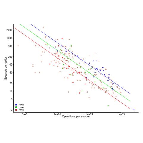
The fitted exponent for this form of x/y axis maps to a value which has , i.e., there are economies of scale.
It so happens that the value of the Knight’s fitted exponent is close to that proposed in a 1953 paper (“High speed arithmetic: The digital computer as a research tool”, no online copy):
It used to cost one cent to do a multiplication on a desk calculator; now it is more like four cents; but with these big machines we can do a million in an hour for $400, and that means twenty-five multiplications for a cent! I believe that there is a fundamental rule, which I modestly call Grosch's law, giving added economy only as the square root of the increase in speed-that is, to do a calculation ten times as cheaply you must do it one hundred times as fast. |
which did indeed become widely known as Grosch’s law.
Having been given a lucky kick-start by Knight (fitted individually, years are not close to Grosch’s law), checking for agreement with Grosch’s law became a focus for later studies. While various papers highlighted problems with the later data analysis (e.g., the regression techniques and sample noise producing mathematical artifacts), Grosch’s law ceased being a thing because mainframes/minicomputers ceased being a thing.
Did mainframe/mincomputers have economies of scale in the years after Knight’s data? It’s difficult to tell, the publicly available data is too sparse to support reliable analysis.
Data+code for book: The New C Standard
All the data+code from my book The New C Standard: An Economic and Cultural Commentary is now available on GitHub. For many years I have been meaning to create an easy way to map from a graph/table in the book to the file containing the data, which has blocked me adding the data to GitHub. I have unblocked by releasing this minimal viable product, i.e., it is essentially a copy of the usage subdirectory in the book’s directory.
While the five stage process to get from graph/table to data is tedious, at least there is a process that provides the data. The caption of the graphs in my Evidence-based Software Engineering book contain a link to the corresponding file on GitHub. This was not possible for the C book because GitHub was still 3-years in the future when the book was published (in 2005).
Work on the book started in late 1999 and measurements of C usage was an integral component. Publicly available source code was still a novelty and large Open source projects were rare (SourceForge was launched at the end of 1999). The large projects with C source available to measure were: Linux, Netscape, Gcc, PostgresSQL, OpenAFS, and OpenMotif. Several popular projects originally written in C had migrated to using C++, and were therefore not applicable.
As the book was completed in 2005, evidence-based software engineering restarted, 20-years after the fall of Rome. Or rather, I have nominated 2005 as the year this happened. Feel free to quibble plus/minus a few years.
Search engines were an essential tool for obtaining research papers, reports, and occasionally downloading data. In 2000 the search engine of choice was AltaVista, but a few years later Google had become the best.
While writing the book, I was a regular visitor to bricks and mortar buildings called libraries. Back then, university libraries contained tens of thousands of physical books, and researchers would photocopy papers of interest. Little did I know that this research practice would soon be dead.
In 2005, I had this to say about software evolution:
Measuring the characteristics of software that change over many releases (software evolution) is a relatively new research topic. Software evolution is discussed in a few sentences, and any future major revision ought to cover this important topic in substantially more detail. |
How might C source code characteristics have changed in the last 20 years?
- The use of K&R style function definitions is probably very rare; it was well on the way out in 1999,
- big software systems have gotten bigger, i.e., more lines of code and more
#includes, - A lot more code using 32-bit integers and 64-bit pointers,
- More storage allocated (memory capacity has increased) because it’s faster to do everything in memory, and there is more data.
Distribution of integer literals in text/speech and source code
Numeric values are an integral to communication between people. What is the distribution of integer values in text/speech, and does the use of integer literals in source code have a similar distribution?
- The paper Numbers in Context: Cardinals, Ordinals, and Nominals in American English by Greg Woodin, and Bodo Winter studied the 9+ million numbers contained in the Corpus of Contemporary American English (7,744,038 integer values). The plot below shows the number of occurrences of the smaller integer values, and a fitted regression line for values in the range 1..50 (code+data):

The frequency of integer values in this corpus is proportional to:
 .
. - The paper Frequency of occurrence of numbers in the World Wide Web by Dorogovtsev, Mendes, and Gama Oliveira found that the number of web pages containing a given integer value declines as the value increases, with the decline for non-round numbers being roughly proportional to
 (round numbers are much more frequent than adjacent values and bias fitted models), and including all values gives
  (for values up to
  ).
).
Programs are an implementation of a sliver of the world in which people live, and it is to be expected that the frequency of numeric literal values in source code is highly correlated with real world frequency. Numeric values also appear in the algorithms and mathematical expressions used to create implementations. I am not aware of any studies looking at the frequency of use of numeric constants in algorithms and mathematics. As an aside, the frequency of occurrence of mathematical expressions containing a given number of operators is similar to that in C source
What are the usage characteristics of integer literals in source code (floating-point literal use is very rare outside of particular application domains)?
The plot below shows occurrences of decimal (green) and hexadecimal (blue) literals in C source (data from fig 825.1 from my C book) with a regression line fitted to values 1..50 of the decimal data (code+data):

The frequency of decimal literal values in C source is proportional to: . Adding the hexadecimal values to the model has little effect.
The paper What do developers consider magic literals? A smalltalk perspective by Anquetil, Delplanque, Ducasse, Zaitsev, Fuhrman, and Guéhéneuc studied the use of literals in Smalltalk. The plot below shows the number of occurrences of all kinds of integer literals and a fitted regression line (code+data):

The frequency of integer literal values in Smalltalk source is proportional to:  .
.
The distribution of integer literals in both human communication and source code is well-fitted by a power law. Smalltalk appears to be the outlier, with an exponent of 1.7 vs 1.3-1.4. Perhaps it’s a sample size issue; 14,054 integer literals for Smalltalk and a million+ for the other datasets.
I had expected source code to contain a lot more zeroes/ones, relative to other values, than human communication. Zero/one are such common values that there are implicit short-cuts that people can use to express them; removing the effort/cost needed to explicitly specify them. Some programming languages specify default 0/1 values for common idioms, but C-like languages generally require explicit specification of values.
ISO C++ committee has a new chief sheep herder
The ISO C++ Standards committee, WG21, has a new convenor, Guy Davidson, or rather they will have when the term of the current convenor, Herb Sutter, expires at the end of this year.
Apart from the few people directly involved, this appointment does not matter to anybody (sorry Guy). The WG21 juggernaut will continue on its hedonistic way, irrespective of who is currently the chief sheep herder.
Before discussing the evolution of language standards, a brief summary of the unusual points around this appointment:
- More than one person volunteered for the job (several in the US, who selected Jeff Garland, and one in the UK; everyone agreed that both were capable candidates). The announcement by a programming language convenor that they are not standing again when their 3-year term expires more commonly kicks off discrete discussions about whose arm can be twisted to take on the role. It’s a thankless task that consumes time and money (to attend extra meetings). Also, the convenor has to be neutral, which circumscribes being involved in technical discussion.
Sometimes an outsider pops up, ruffles a few feathers and then disappears (from the Standards’ world).
- One of the SC22 (the ISO committee responsible for programming languages) convenor selection rules says (see Resolution 14-04): “When a WG Convenorship becomes vacant, … and multiple NBs have each nominated a candidate, the Convenorship shall be assigned to the candidate whose NB currently has the fewest SC 22 Convenors.” Currently, the US holds multiple convenorships and the UK holds none, so the UK nominee is appointed.
As often happens, people like diversity rules until they lose out. The US submitted a selection procedural change to SC22, and asked that it take effect before the selection of a new WG21 convenor. The overwhelming consensus at the SC22 plenary last Monday was not to change the rules while an election was in progress. An ad-hoc committee was set up to consider changes to the current rules.
End of the news and back to regular postings.
Standards committees for programming languages are now a vestige from a bygone era. The original purpose of standards was to reduce costs (the UK focused on savings achieved through repeated use of standardized items and the US focused on reduced training costs) by having companies manufacture products that conformed to a single specification.
There were once a multitude of implementations for the commercially important languages, each supporting slightly different dialects (the differences were sometimes not so slight). Language standards provided a base specification for developers interested in portable code to keep within, and that vendors could be pressured to support.
The spread of Open source compilers significantly reduced the need for companies to invest in maintaining their own compiler (there might be strategic reasons for companies selling hardware or operating systems to continue to invest in their own compiler), and reduced the likelihood that customers of commercial compiler companies would continue to pay for updates (effectively driving most compiler companies out of business).
Language standards are redundant in a monoculture, i.e., where only one compiler per language is widely used. For some years now, there have been a handful of actively maintained compilers for the widely used languages.
These days, conformance to a language standard is measured by the ability of an implementation to compile and execute the Open source software available in the various ecosystems.
As has often been observed, committees find work to keep themselves busy, and I have seen announcements for new ISO committees that look like they were created because somebody saw a CV padding opportunity.
I continue to think that the C++ committee has become a playground for bored consultants looking for a creative outlet.
WG21 meeting attendance continues to grow, now attracting 200+ attendees (Grok undercounts, e.g., 140 vs 215, and ChatGPT 5 is completely out of its depth). This is an order of magnitude greater than the C committee, WG14, and in a few years could be two orders of magnitude greater than the other SC22 languages.
The two major C/C++ compiler vendors (i.e., gcc and llvm) could simply go their own way, with regard to new language features. However, I imagine that “supporting the latest version of the language standard” is a great rationale to use when asking for funding.
How large can WG21 become before it collapses under the weight of members and the papers they write?
The POSIX standard, WG15, meetings often had 200-300 attendees in the late 1980s/early 1990s. But the POSIX committee stuck to its goal of specifying existing practice, and so has faded away.
Guy strikes me as an efficient administrator. Which is probably bad news, in the sense that this could enable WG21 to grow a lot larger. What ever happens, it will be interesting to watch.
Percentage of methods containing no reported faults
It is often said, with some evidence, that 80% of reported faults, for a program, occur in 20% of its code. I think this pattern is a consequence of 20% of the code being executed 80% of the time, while many researchers believe that 20% of the source code has characteristics that result in it containing 80% of the coding mistakes.
The 20% figure is commonly measured as a percentage of methods/functions, rather than a percentage of lines of code.
This post investigates the expected fraction of a program’s methods that remain fault report free, based on two probability models.
Both models assume that coding mistakes are uniformly scattered throughout the code (i.e., every statement has the same probability of containing a mistake) and that the corresponding coding mistake is contained within a single method (the evidence suggests that this is true for 50% of faults).
A simple model is to assume that when a new fault is reported, the probability that the corresponding coding mistake appears in a particular method is proportional to the method’s length,  in lines of code, of the method. The evidence shows that the distribution of methods containing a given number of lines, , is well-fitted by a power law (for Java:
  ).
).
If  reported faults have been fixed in a program containing
  methods/functions, what is the expected number of methods that have not been modified by the fixing process?
The answer (with help from: mostly Kimi, with occasional help from Deepseek (who don’t have a share chat options), ChatGPT 5, Grok, and some approximations; chat logs) is:
}Li_b(e^{-{F/M}{{zeta(b)}/{zeta(b-1)}}})")
where:  is the Riemann zeta function,
  is the polylogarithm function and
  for Java.
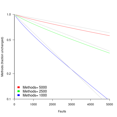
The plot below shows the predicted fraction of unmodified methods against number of faults, for programs of various sizes; the grey lines show the rough approximation:  (code+data):
The observed behavior of most reported faults involving a subset of a program’s methods can be modelled using some form of preferential attachment.
One preferential attachment model specifies that the likelihood of a coding mistake appearing in a method is proportional to ") , where is the number of previously detected coding mistakes in the method.
, where is the number of previously detected coding mistakes in the method.
The estimated number of unmodified methods is now:
}Li_b(({M zeta(b-1)}/{M zeta(b-1)+a*(F+1) zeta(b)})^{1/a})")
where: is the average value of  over all faults (if
  , then
  for a power law with exponent 2.35).
The plot below shows the predicted fraction of unmodified methods against number of faults for a program containing 1,000 methods, for various values of , with the black line showing the fraction of unmodified methods predicted by the simple model above (code+data):
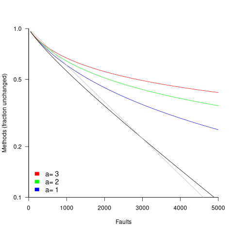
In practice, random selection of the method containing a coding mistake will introduce some fuzziness in the predicted fraction of unmodified methods.
As the number of reported faults grows, the attraction of methods involved in previous reported faults slows the rate at which methods experience their first detected coding mistake.
How realistic are these models?
By focusing on the number of unmodified methods, many complications are avoided.
Both models assume that an unchanging number of methods in a program and that the length of each method is fixed. This assumption holds between each release of a program.
For actively maintained programs, the number of methods in a program changes over time, and the length of some existing methods also changes (if a program were not actively maintained, reported faults would not get fixed).
These models are unlikely to be applicable to programs with short release cycles, where there are few reported faults between releases.
How well do the models’ predictions agree with the data?
At the moment, I am not aware of a dataset containing the appropriate data. Number of faults vs unmodified methods has been added to my list of interesting patterns to notice.
Summary of the derivation of the solutions for the two models.
Simple model
The expected number of unmodified methods, ") , is:
, is:
=sum{L=1}{T}{m_L{P(U_LF)}}") , where
, where  is the length of the longest method,
  is the number of methods of length , and
 ") is the probability that a method of length will be unmodified after fault reports.
is the probability that a method of length will be unmodified after fault reports.
The evidence shows that the distribution of methods containing a given number of lines, , is well-fitted by a power law (for Java: ).
Given a program containing methods, the number of methods of length is:
 , where for Java.
If is large and  , then the sum can be approximated by the Riemann zeta function, , giving:
}}")
The probability that a method containing lines will not be modified by a fault report (assuming that fixing the mistake only involves one method) is:  , where
  is the total lines of code in the program, and the probability of this method not being modified after fault reports is approximately:
^F approx e^{{-F*L}/{P_t}}")
The expected number of empty boxes is:
}}*e^{{-F*L}/{P_t}}}=M/{zeta(b)}Li_b(e^{-F/{P_t}})")
The number of lines of code in a program containing methods is:
}}}=M/{zeta(b)}sum{L=1}{T}{L^{1-b}}=M{{zeta(b-1)}/{zeta(b)}}")
Finally giving:
}Li_b(e^{-{F/M}{{zeta(b)}/{zeta(b-1)}}})")
where is the polylogarithm function.
This equation is roughly, for the purposes of understanding the effect of each variable:

Preferential attachment model
When a mistake is corrected in a method, the attraction weight of that method increases (alternatively, the attraction weight of the other methods decreases). The probability that a method is not modified after fault reports is now:
}=prod{k=0}{F}{{P_t+a*k-L}/{P_t+a*k}}={Gamma({P_t}/a)Gamma({P_t-L}/a+F+1)}/{Gamma({P_t-L}/a)Gamma(P_t/a+F+1)}")
where:  the average value of over all faults, and
  is the gamma function.
applying the Stirling/Gamma–ratio rule, i.e., }/{Gamma(z+b)} approx z^{a-b}") we get:
we get:
})^{F/a} = ((P_t/{P_t+a*(F+1)})^{1/a})^F")
where the expression ^{1/a})^F") is the preferential attachment version of the expression
is the preferential attachment version of the expression ^F") appearing in the simple model derivation. Using this preferential attachment expression in the analysis of the simple model, we get:
appearing in the simple model derivation. Using this preferential attachment expression in the analysis of the simple model, we get:
I don’t have a rough approximation for this expression.
Halstead/McCabe: a complicated formula for LOC
My experience is that people prefer to ignore the implications of Halstead’s metric and McCabe’s complexity metric being strongly correlated (non-linearly) with lines of code (LOC). The implications being that they have been deluding themselves and perhaps wasting time/money using Halstead/McCabe when they could just as well have used LOC.
If the purpose of collecting metrics is a requirement to tick a box, then it does not really matter which metrics are collected. The Halstead/McCabe metrics have a strong brand, so why not collect them.
Don’t make the mistake of thinking that Halstead/McCabe is more than a complicated way of calculating LOC. This can be shown by replacing Halstead/McCabe by the corresponding LOC value to find that it makes little difference to the value calculated.
Some metrics include the Halstead metrics and/or the McCabe metric as part of their calculation. The Maintainability Index is a metric calculated using Halstead’s volume, McCabe’s complexity and lines of code. Its equation is (see below for details):
-0.23*McCabe-16.2*ln(LOC)")
Replacing the Halstead/McCabe terms by one involving just LOC requires an appropriate mapping. Nearly all researchers assume a linear mapping, despite the overwhelming evidence that the mapping is non-linear.
Fitting regression models for HalsteadVolume vs LOC and McCabe vs LOC, using measurements of 730K methods from 47 Java projects (see below for data details), produces the coefficients for the equation needed to map each metric to LOC (previous analysis has found that a power law provides the best mapping; code+data). Substituting these equations in the Maintainability Index equation above, we get:
)-0.23*(0.45*LOC^{0.71})-16.2*ln(LOC)")
which simplifies to:
-0.1*LOC^{0.71}")
How does the value calculated using  compare with the corresponding
  value?
For 99.7% of methods, the relative error,  , for the 730K Java methods is less than 10%, and for 98.6% of methods the relative error is less than 5% (code+data).
Given the fuzzy nature of these metrics, 10% is essentially noise.
Looking at the relative contributions made by Halstead/McCabe/LOC to the value of the Maintainability Index, second equation above, the Halstead contribution is around a third the size of the LOC contribution and the McCabe contribution is at least an order of magnitude smaller.
Background on the Maintainability Index and the measured Java projects.
The Maintainability Index was introduced in the 1994 paper “Construction and Testing of Polynomials Predicting Software Maintainability” by Oman, and Hagemeister (270 citations; no online pdf), a 1992 paper by the same authors is often incorrectly cited (426 citations). The earlier 1992 paper identified 92 known maintainability attributes, along with 60 metrics for “… gauging software maintainability …” (extracted from 35 published papers).
This Maintainability Index equation was chosen from “Approximately 50 regression models were constructed and tested in our attempts to identify simple models that could be calculated from existing tools and still be generic enough to be applied to a wide range of software.” The data fitted came from eight suites of programs (average LOC 3,568 per suite), along “… with subjective engineering assessments of the quality and maintainability of each set of code.”
Yes, choosing from 50 regression models looks like overfitting, and by today’s standards 28.5K LOC is a tiny amount of source.
The data used is distributed with the paper Revisiting the Debate: Are Code Metrics Useful for Measuring Maintenance Effort? by Chowdhury, Holmes, Zaidman, and Kazman, which does a good job of outlining the many different definitions of maintenance and the inconsistent results from prediction models. However, the authors remain under the street light of project source code, i.e., they ignore the fact that many maintenance requests are driven by demand for new features.
The authors investigate the impact of normalizing Halstead/McCabe by LOC, but make the common mistake of assuming a linear relationship. They are surprised by the high correlation between post-‘normalised’ Halstead/McCabe and LOC. The correlation disappears when the appropriate non-linear normalization is used; see code+data.
A 2014 paper by Najm also maps the components of the Maintainability Index to LOC, but uses a linear mapping from the Halstead/McCabe terms to LOC, creating a equation whose behavior is noticeably different.
Half-life of Open source research software projects
The evidence for applications having a half-life continues to spread across domains. The first published data covered IBM mainframe applications up to 1992 (half-life of at least 5-years), and was mostly ignored. Then, the data collected by Killed by Google up to 2018, showed a half-life of at least 3-years for Google apps. More recently, the data collected by Killed by Microsoft up to 2025, showed a half-life of at least 7-years for Microsoft apps (perhaps reflecting the maturity of the company’s product line).
The half-life of source code, independent of the lifetime of the application it implements, is a separate topic.
Scientific software created to support researchers is an ecosystem whose incentives and means of production can be very different from commercial software. Does researcher oriented software die when the grant money runs out, or the researcher moves on to the next fashionable topic, or does it live on as the field expands?
The paper Scientific Open-Source Software Is Less Likely to Become Abandoned Than One Might Think! Lessons from Curating a Catalog of Maintained Scientific Software by Thakur, Milewicz, Jahanshahi, Paganini, Vasilescu, and Mockus analysed 14,418 scientific software systems written in Python (53%), C/C++ (25%), R (12%), Java (8%) or Fortran (2%). The first half of the paper describes how World of Code‘s 209 million repos were filtered down to 350,308 projects containing README files, these READMEs were processed by LLMs to extract information and further filter out projects.
The authors collected the usual information about each Open source project, e.g., number of core developers, number of commits, programming language, etc. They also collected information about the research domain, e.g., scientific field (biology, chemistry, mathematics, etc.), funding, academic/government associations, etc. A Cox proportional hazards model was fitted to this data, with project lifetime being the response variable. A project was deemed to have been abandoned when no changes had been made to the code for at least six consecutive months (we can argue over whether this is long enough).
Including all the different factors created a Cox model that did a good job of explaining the variance in project survival rate. No one factor dominated, and there was a lot of overlap in the confidence bounds of the components of each factor, e.g., different research domains. I have always said that programming language has no impact on project lifetime; the language factor of the fitted model was not statistically significant (two of the languages just sneaked in under the 5% bar), which can be interpreted as being consistent with my opinion.
Each project was categorised as one of: Scientific Domain-specific code (73.5%), Scientific infrastructure (16.5%), or Publication-Specific code (10%). The plot below shows the Kaplan-Meier survival curve for these three categories (note: y-axis is logarithmic), with faint grey lines showing a fitted exponential for each survival curve (only 3% of projects are abandoned in the first year, and the exponential fits are to the data after the first year; code+data):
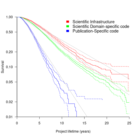
Readers familiar with academic publishing will not be surprised that projects associated with published papers have the lowest survival rate (half-life just over 2-years). Infrastructure projects are likely to be depended on by many people, who all have an interest in them surviving (half-life around 6-years). The Domain-specific half-life is around 4.5-years.
The results of this study show software systems in various research ecosystems having a range of half-lives in the same range as three major commercial software ecosystems.
Unfortunately, my experience of discussing application half-life with developers is that they believe in an imagined future where software never dies. That is, they are unwilling to consider a world where software has a high probability of being abandoned, because it requires that they consider the return on investment before spending time polishing their code.
Positive and negative descriptions of numeric data
Effective human communication is based on the cooperative principle, i.e., listeners and speakers act cooperatively and mutually accept one another to be understood in a particular way. However, when seeking to present a particular point of view, speakers may prefer to be economical with the truth.
To attract citations and funding, researchers sell their work via the papers they publish (or blogs they write), and what they write is not subject to the Advertising Standards Authority rule that “no marketing communication should mislead, or be likely to mislead, by inaccuracy, ambiguity, exaggeration, omission or otherwise” (my default example).
When people are being economical with the truth, when reporting numeric information, are certain phrases or words more likely to be used?
The paper: Strategic use of English quantifiers in the reporting of quantitative information by Silva, Lorson, Franke, Cummins and Winter, suggests some possibilities.
In an experiment, subjects saw the exam results of five fictitious students and had to describe the results in either a positive or negative way. They were given a fixed sentence and had to fill in the gaps by selecting one of the listed words; as in the following:
             all                      all
             most                     most                  right
In this exam .... of the students got .... of the questions .....
             some                     some                  wrong
none none |
If you were shown exam results with 2 out of 5 students failing 80% of questions and the other 3 out of 5 passing 80% of questions, what positive description would you use, and what negative description would you use?
The 60 subjects each saw 20 different sets of exam results for five fictitious students. The selection of positive/negative description was random for each question/subject.
The results found that when asked to give a positive description, most responses focused on questions that were right, and when asked to give a negative description, most responses focused on questions that were wrong
How many questions need to be answered correctly before most can be said to be correct? One study found that at least 50% is needed.
“3 out of 5 passing 80%” could be described as “… most of the students got most of the questions right.”, and “2 out of 5 students failing 80%” could be described as “… some of the students got most of the questions wrong.”
The authors fitted a Bayesian linear mixed effect models, which showed a somewhat complicated collection of connections between quantifier use and exam results. The plots below provide a visual comparison of the combination of quantifier use for positive (upper) and negative (lower) descriptions.
The alluvial plot below shows the percentage flow, for Positive descriptions, of each selected quantifier through student and question, and then adjective (code+data):

For the same distribution of exam results, the alluvial plot below shows the percentage flow, for Negative descriptions, of each selected quantifier through student and question, and then adjective (code+date):
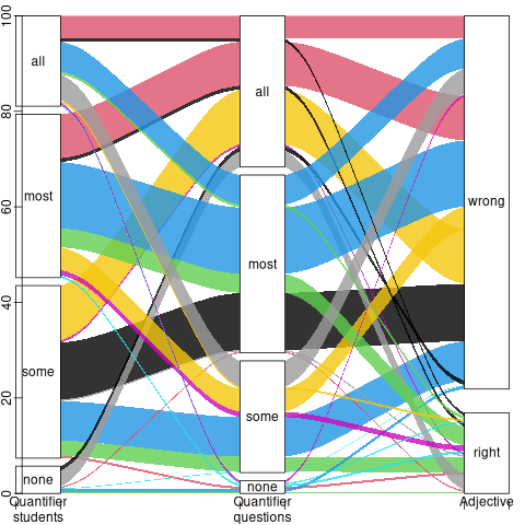
Other adjectives could be used to describe the results (e.g., few, several, many, not many, not all), and we will have to wait for the follow-up research to this 2024 paper.
Predicted impact of LLM use on developer ecosystems
LLMs are not going to replace developers. Next token prediction is not the path to human intelligence. LLMs provide a convenient excuse for companies not hiring or laying off developers to say that the decision is driven by LLMs, rather than admit that their business is not doing so well
Once the hype has evaporated, what impact will LLMs have on software ecosystems?
The size and complexity of software systems is limited by the human cognitive resources available for its production. LLMs provide a means to reduce the human cognitive effort needed to produce a given amount of software.
Using LLMs enables more software to be created within a given budget, or the same amount of software created with a smaller budget (either through the use of cheaper, and presumably less capable, developers, or consuming less time of more capable developers).
Given the extent to which companies compete by adding more features to their applications, I expect the common case to be that applications contain more software and budgets remain unchanged. In a Red Queen market, companies want to be perceived as supporting the latest thing, and the marketing department needs something to talk about.
Reducing the effort needed to create new features means a reduction in the delay between a company introducing a new feature that becomes popular, and the competition copying it.
LLMs will enable software systems to be created that would not have been created without them, because of timescales, funding, or lack of developer expertise.
I think that LLMs will have a large impact on the use of programming languages.
The quantity of training data (e.g., source code) has an impact on the quality of LLM output. The less widely used languages will have less training data. The table below lists the gigabytes of source code in 30 languages contained in various LLM training datasets (for details see The Stack: 3 TB of permissively licensed source code by Kocetkov et al.):
Language TheStack CodeParrot AlphaCode CodeGen PolyCoder HTML 746.33 118.12 JavaScript 486.2 87.82 88 24.7 22 Java 271.43 107.7 113.8 120.3 41 C 222.88 183.83 48.9 55 C++ 192.84 87.73 290.5 69.9 52 Python 190.73 52.03 54.3 55.9 16 PHP 183.19 61.41 64 13 Markdown 164.61 23.09 CSS 145.33 22.67 TypeScript 131.46 24.59 24.9 9.2 C# 128.37 36.83 38.4 21 GO 118.37 19.28 19.8 21.4 15 Rust 40.35 2.68 2.8 3.5 Ruby 23.82 10.95 11.6 4.1 SQL 18.15 5.67 Scala 14.87 3.87 4.1 1.8 Shell 8.69 3.01 Haskell 6.95 1.85 Lua 6.58 2.81 2.9 Perl 5.5 4.7 Makefile 5.09 2.92 TeX 4.65 2.15 PowerShell 3.37 0.69 FORTRAN 3.1 1.62 Julia 3.09 0.29 VisualBasic 2.73 1.91 Assembly 2.36 0.78 CMake 1.96 0.54 Dockerfile 1.95 0.71 Batchfile 1 0.7 Total 3135.95 872.95 715.1 314.1 253.6 |
The major companies building LLMs probably have a lot more source code (as of July 2023, the Software Heritage had over  unique source code files); this table gives some idea of the relative quantities available for different languages, subject to recency bias. At the moment, companies appear to be training using everything they can get their hands on. Would LLM performance on the widely used languages improve if source code for most of the 682 languages listed on Wikipedia was not included in their training data?
Traditionally, developers have had to spend a lot of time learning the technical details about how language constructs interact. For the first few languages, acquiring fluency usually takes several years.
It’s possible that LLMs will remove the need for developers to know much about the details of the language they are using, e.g., they will define variables to have the appropriate type and suggest possible options when type mismatches occur.
Removing the fluff of software development (i.e., writing the code) means that developers can invest more cognitive resources in understanding what functionality is required, and making sure that all the details are handled.
Removing a lot of the sunk cost of language learning removes the only moat that some developers have. Job adverts could stop requiring skills with particular programming languages.
Little is currently known about developer career progression, which means it’s not possible to say anything about how it might change.
Since they were first created, programming languages have fascinated developers. They are the fashion icon of software development, with youngsters wanting to program in the latest language, or at least not use the languages used by their parents. If developers don’t invest in learning language details, they have nothing language related to discuss with other developers. Programming languages will cease to be a fashion icon (cpus used to be a fashion icon, until developers did not need to know details about them, such as available registers and unique instructions). Zig could be the last language to become fashionable.
I don’t expect the usage of existing language features to change. LLMs mimic the characteristics of the code they were trained on.
When new constructs are added to a popular language, it can take years before they start to be widely used by developers. LLMs will not use language constructs that don’t appear in their training data, and if developers are relying on LLMs to select the appropriate language construct, then new language constructs will never get used.
By 2035 things should have had time to settle down and for the new patterns of developer behavior to be apparent.
Recent Comments