Archive
CPU power consumption and bit-similarity of input
Changing the state of a digital circuit (i.e., changing its value from zero to one, or from one to zero) requires more electrical power than leaving its state unchanged. During program execution, the power consumed by each instruction depends on the value of its operand(s). The plot below, from an earlier post, shows how the power consumed by an 8-bit multiply instruction varies with the values of its two operands:
An increase in cpu power consumption produces an increase in its temperature. If the temperature gets too high, the cpu’s DVFS (dynamic voltage and frequency scaling) will slow down the processor to prevent it overheating.
When a calculation involves a huge number of values (e.g., an LLM size matrix multiply), how large an impact is variability of input values likely to have on the power consumed?
The 2022 paper: Understanding the Impact of Input Entropy on FPU, CPU, and GPU Power by S. Bhalachandra, B. Austin, S. Williams, and N. J. Wright, compared matrix multiple power consumption when all elements of the matrices had the same values (i.e., minimum entropy) and when all elements had different random values (i.e., maximum entropy).
The plot below shows the power consumed by an NVIDIA A100 Ampere GPU while multiplying two 16,384 by 16,384 matrices (performed 100 times). The GPU was power limited to 400W, so the random value performance was lower at 18.6 TFLOP/s, against 19.4 TFLOP/s for same values; (I don’t know why the startup times differ; code+data):
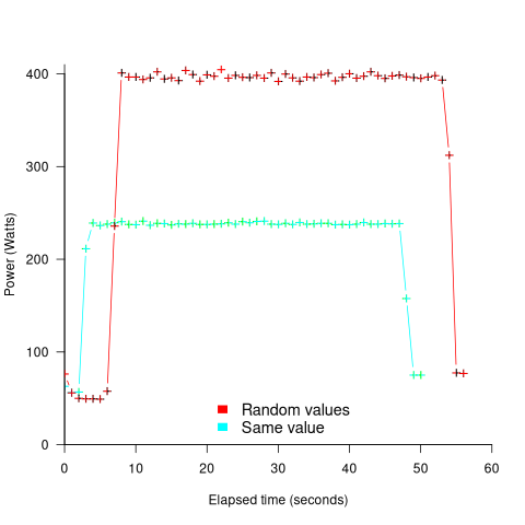
This 67% performance difference is more than an interesting factoid. Large computations are distributed over multiple GPUs, and the output from each GPU is sometimes feed as input to other GPUs. The flow of computations around a cluster of GPUs needs to be synchronised, and having compute time depend on the distribution of the input values makes life complicated.
Is it possible to organise a sequence of calculation to reduce the average power consumed?
The higher order bits of small integers are zero, but how many long calculations involve small integers? The bit pattern of floating-point values are more difficult to predict, but I’m sure there is a PhD thesis or two waiting to be written around this issue.
Procedure nesting a once common idiom
Structured programming was a popular program design methodology that many developers/managers claimed to be using in the 1970s and 1980s. Like all popular methodologies, everybody had/has their own idea about what it involves, and as always, consultancies sprang up to promote their take on things. The 1972 book Structured programming provides a taste of the times.
The idea underpinning structured programming is that it’s possible to map real world problems to some hierarchical structure, such as in the image below. This hierarchy model also provided a comforting metaphor for those seeking to understand software and its development.

The disadvantages of the Structured programming approach (i.e., real world problems often have important connections that cannot be implemented using a hierarchy) become very apparent as programs get larger. However, in the 1970s the installed memory capacity of most computers was measured in kilobytes, and a program containing 25K lines of code was considered large (because it was enough to consume a large percentage of the memory available). A major program usually involved running multiple, smaller, programs in sequence, each reading the output from the previous program. It was not until the mid-1980s…
At the coding level, doing structured programming involves laying out source code to give it a visible structure. Code blocks are indented to show if/for/while nesting and where possible procedure/functions are nested within the calling procedures (before C became widespread, functions that did not return a value were called procedures; Fortran has always called them subroutines).
Extensive nesting of procedures/functions was once very common, at least in languages that supported it, e.g., Algol 60 and Pascal, but not Fortran or Cobol. The spread of C, and then C++ and later Java, which did not support nesting (supported by gcc as an extension, nested classes are available in C++/Java, and later via lambda functions), erased nesting from coding consideration. I started life coding mostly in Fortran, moved to Pascal and made extensive use of nesting, then had to use C and not being able to nest functions took some getting used to. Even when using languages that support nesting (e.g., Python), I have not reestablished by previous habit of using nesting.
A common rationale for not supporting nested functions/methods is that it complicate the language specification and its implementation. A rather self-centered language designer point of view.
The following Pascal example illustrates a benefit of being able to nest procedures/functions:
procedure p1; var db :array[db_size] of char; procedure p2(offset :integer); function p3 :integer; begin (* ... *) return db[offset]; end; begin var off_val :char; off_val=p3; (* ... *) end; begin (* ... *) p2(3) end; |
The benefit of using nesting is in not forcing the developer to have to either define db at global scope, or pass it as an argument along the call chain. Nesting procedures is also a method of information hiding, a topic that took off in the 1970s.
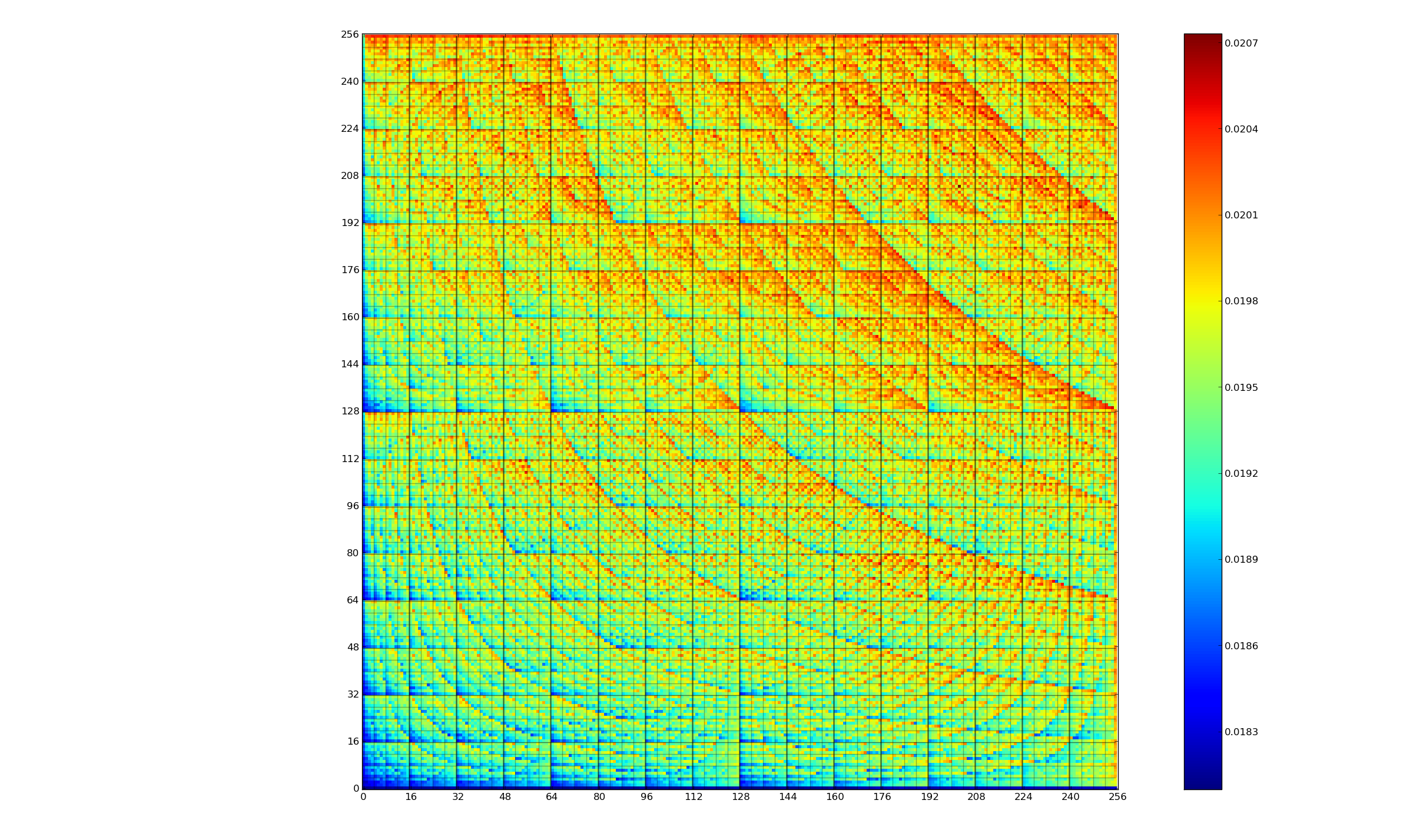
To what extent did Algol/Pascal developers use nested procedures? A 1979 report by G. Benyon-Tinker and M. M. Lehman contains the only data I am aware of. The authors analysed the evolution of procedure usage within a banking application, from 1973 to 1978. The Algol 60 source grew from 35,845 to 63,843 LOC (657 procedures to 967 procedures). A large application for the time, but a small dataset by today’s standards.
The plot below shows the number of procedures/functions having a particular lexical nesting level, with nesting level 1 is the outermost level (i.e., globally visible procedures), and distinct colors denoting successive releases (code+data):

Just over 78% of procedures are nested within at least one other procedure. It’s tempting to think that nesting has a Poisson distribution, however, the distribution peaks at three rather than two. Perhaps it’s possible to fit an over-dispersed, but this feels like creating a just-so story.
What is the distribution of nested functions/methods in more recently written source? A study of 35 Python projects found 6.5% of functions nested and over twice as many (14.2%) of classed nested.
Are there worthwhile benefits to using nested functions/methods where possible, or is this once common usage mostly fashion driven with occasional benefits?
Like most questions involving cost/benefit analysis of language usage, it’s probably not sufficiently interesting for somebody to invest the effort required to run a reliable study.
Functions reduce the need to remember lots of variables
What, if any, are the benefits of adding bureaucracy to a program by organizing a file’s source code into multiple function/method definitions (rather than a single function)?
Having a single copy of a sequence of statements that need to be executed at multiple points in a program reduces implementation effort, and any updates only need to be made once (reducing coding mistakes by removing the need to correctly make duplicate changes). A function/method is the container for this sequence of statements.
Why break code up into separate functions when each is only called once and only likely to ever be called once?
The benefits claimed from splitting code into functions include: making it easier to understand, test, debug, maintain, reuse, and scale development (i.e., multiple developers working on the same program). Our LLM overlords also make these claims, and hallucinate references to published evidence (after three iterations of pointing out the hallucinated references, I gave up asking for evidence; my experience with asking people is that they usually remember once reading something but cannot remember the source).
Regular readers will not be surprised to learn that there is little or no evidence for any of the claimed benefits. I’m not saying that the benefits don’t exist (I think there are some), simply that there have not been any reliable studies attempting to measure the benefits (pointers to such studies welcome).
Having decided to cluster source code into functions, for whatever reason, are there any organizational rules of thumb worth following?
Rules of thumb commonly involve function length (it’s easy to measure) and desirable semantic characteristics of distinct functions (it’s very hard to measure semantic characteristics).
Claims for there being an optimal function length (i.e., lines of code that minimises coding mistakes) turned out to be driven by a mathematical artifact of the axis used when plotting (miniscule) datasets.
Semantic rules of thumb such as: group by purpose, do one thing, and Single-responsibility principle are open to multiple interpretations that often boil down to personal preferences and experience.
One benefit of using functions that is rarely studied is the restricted visibility of local variables defined within them, i.e., only visible within the function body.
When trying to figure out what code does, readers have to keep track of the information contained in all the variables accessed. Having to track more variables not only increases demands on reader memory, it also increases the opportunities for making mistakes.
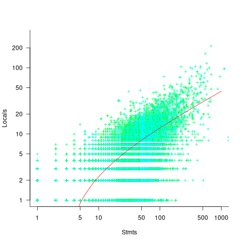
A study of C source found that within a function, the number of local variables is proportional to the square root of the number of statements (code+data). Assuming the proportionality constant is one, a function containing 100 statements might be expected to define 10 local variables. Splitting this function up into, say, four functions containing 25 statements, each is expected to define 5 local variables. The number of local variables that need to be remembered at the same time, when reading a function definition, has halved, although the total number of local variables that need to be remembered when processing those 100 statements has doubled. Some number of global variables and function parameters need to be added to create an overall total for the number of variables.
The plot below shows the number of locals defined in 36,617 C functions containing a given number of statements, the red line is a fitted regression model having the form:  (code+data):
My experience with working with recently self-taught developers, especially very intelligent ones, is that they tend to write monolithic programs, i.e., everything in one function in one file. This minimal bureaucracy approach minimises the friction of a stream of thought development process for adding new code, and changing existing code as the program evolves. Most of these programs are small (i.e., at most a few hundred lines). Assuming that these people continue to code, one of two events teaches them the benefits of function bureaucracy:
- changes to older programs becomes error-prone. This happens because the developer has forgotten details they once knew, e.g., they forget which variables are in use at particular points in the code,
- the size of a program eventually exceeds their ability to remember all of it (very intelligent people can usually remember much larger programs than the rest of us). Coding mistakes occur because they forget which variables are in use at particular points in the code.
Remotivating data analysed for another purpose
The motivation for fitting a regression model has a major impact on the model created. Some of the motivations include:
- practicing software developers/managers wanting to use information from previous work to help solve a current problem,
- researchers wanting to get their work published seeks to build a regression model that show they have discovered something worthy of publication,
- recent graduates looking to apply what they have learned to some data they have acquired,
- researchers wanting to understand the processes that produced the data, e.g., the author of this blog.
The analysis in the paper: An Empirical Study on Software Test Effort Estimation for Defense Projects by E. Cibir and T. E. Ayyildiz, provides a good example of how different motivations can produce different regression models. Note: I don’t know and have not been in contact with the authors of this paper.
I often remotivate data from a research paper. Most of the data in my Evidence-based Software Engineering book is remotivated. What a remotivation often lacks is access to the original developers/managers (this is often also true for the authors of the original paper). A complicated looking situation is often simplified by background knowledge that never got written down.
The following table shows the data appearing in the paper, which came from 15 projects implemented by a defense industry company certified at CMMI Level-3.
Proj  Test    Req   Test Meetings Faulty    Actual Scenarios
      Plan    Rev   Env          Scenarios  Effort
      Time          Time
P1    144.5  1.006    85     60     100      2850    270
P2     25.5  1.001    25.5    4       5       250     40
P3     68    1.005    42.5   32      65      1966    185
P4     85    1.002    85    104     150      3750    195
P5    198    1.007   123     87     110      3854    410
P6     57    1.006    35     25      20       903    100
P7    115    1.003    92     55      56      2143    225
P8     81    1.009   156     62      72      1988    287
P9    388    1.004   150    208     553     13246   1153
P10   177    1.008    93     77     157      4012    360
P11    62    1.001   175    186     199      5017    310
P12   111    1.005   116     82     143      3994    423
P13    63    1.009   188    177     151      3914    226
P14    32    1.008    25     28       6       435     63
P15 167 1.001 177 143 510 11555 1133 |
where: TestPlanTime is the test plan creation time in hours, ReqRev is the test/requirements review of period in hours, TestEnvTime is the test environment creation time in hours, Meetings is the number of meetings, FaultyScenarios is the number of faulty test scenarios, Scenarios is the number of Scenarios, and ActualEffort is the actual software test effort.
Industrial data is hard to obtain, so well done to the authors for obtaining this data and making it public. The authors fitted a regression model to estimate software test effort, and the model that almost perfectly fits to actual effort is:
ActualEffort=3190 + 2.65*TestPlanTime
            -3170*ReqRevPeriod - 3.5*TestEnvTime
+10.6*Meetings + 11.6*FaultScrenarios + 3.6*Scenarios |
My reading of this model is that having obtained the data, the authors felt the need to use all of it. I have been there and done that.
Why all those multiplication factors, you ask. Isn’t ActualTime simply the sum of all the work done? Yes it is, but the above table lists the work recorded, not the work done. The good news is that the fitted regression models shows that there is a very high correlation between the work done and the work recorded.
Is there a simpler model that can be used to explain/predict actual time?
Looking at the range of values in each column, ReqRev varies by just under 1%. Fitting a model that does not include this variable, we get (a slightly less perfect fit):
ActualEffort=100  + 2.0*TestPlanTime
                              - 4.3*TestEnvTime
+10.7*Meetings + 12.4*FaultScrenarios + 3.5*Scenarios |
Simple plots can often highlight patterns present in a dataset. The plot below shows every column plotted against every other column (code+data):

Points forming a straight line indicate a strong correlation, and the points in the top-right ActualEffort/FaultScrenarios plot look straight. In fact, this one variable dominates the others, and fits a model that explains over 99% of the deviation in the data:
ActualEffort=550 + 22.5*FaultScrenarios |
Many of the points in the ActualEffort/Screnarios plot are on a line, and adding Meetings data to the model explains just under 99% of the variance in the data:
actualEffort=-529.5
+15.6*Meetings + 8.7*Scenarios |
Given that FaultScrenarios is a subset of Screnarios, this connectedness is not surprising. Does the number of meetings correlate with the number of new FaultScrenarios that are discovered? Questions like this can only be answered by the original developers/managers.
The original data/analysis was interesting enough to get a paper published. Is it of interest to practicing software developers/managers?
In a small company, those involved are likely to already know what these fitted models are telling them. In a large company, the left hand does not always know what the right hand is doing. A CMMI Level-3 certified defense company is unlikely to be small, so this analysis may be of interest to some of its developer/managers.
A usable estimation model is one that only relies on information available when the estimation is needed. The above models all rely on information that only becomes available, with any accuracy, way after the estimate is needed. As such, they are not practical prediction models.
Recent Comments